

Alternating Least Squares (ALS) and Bayesian Personalized Ranking (BPR) models for recommendations
In this post we're going to see how we can build a recommendation engine using the collaborative filtering models Alternating Least Squares and Bayesian Personalized Ranking from the implicit package in Python. We'll see how we can tune their hyperparameters, measure their performance and visualise the item similarities that the model learns.

Contents
Alternating Least Squares (ALS)
This tutorial covers the Alternating Least Squares (ALS) and Bayesian Personalized Ranking (BPR) algorithms for generating recommendations. We'll be using the implicit package in python to do both of these. Both ALS and BPR are collaborative filtering methods as they works on the principle of "wisdom of the crowd", analysing user and item interactions to learn from and create recommendations e.g. "people who liked X also liked Y". Collaborative filtering models analyse the user-item interaction history directly, agnostic of any attributes about the customer or item. This is in contrast to content based models that focus on the specific attributes of the items or users themselves e.g. the genre of a movie or the demographic details of users (e.g., age, gender).
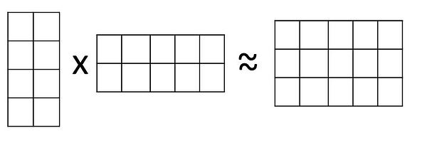
Alternating Least Squares is a matrix factorisation technique that decomposes a user-item interaction matrix into two lower-dimensional matrices: user factors and item factors. This allows for the representation of user preferences and item characteristics in a smaller, latent space. The algorithm is "alternating" because it iteratively fixes item factors to solve for user factors, then fixes user factors to solve for item factors, repeating until convergence. The objective function for implicit feedback in ALS minimizes the squared difference (hence the name 'alternating least squares') between observed preferences and predicted preferences, with a regularization term to prevent overfitting.
Most user-item interaction matrices are sparse in nature, meaning most entries are zero/missing as most users won't have interacted with most items. It's not unusual that out of all the possible user-item interactions in the matrix for over 99% missing! However, by converting this matrix into smaller, dense (i.e. fully populated) factors, when these factors are multiplied together to recreate the original matrix all of the missing values from the original matrix get filled in as well. This is what then allows us to recommend items to customers that they haven't bought before. The dense factors are designed to capture user-item preferences in a condensed manner so that when multiplied they recreate the original user-item interactions found in the original matrix but being dense we also get all of the possible recommendation scores created for us at the same time!
The factors/embeddings themselves can also be incredibly useful as we'll see later. For example, the factors are designed to capture user-item preference in a smaller, shared space. If two customers have very similar purchase behaviours then we'd expect the learnt numerical representation of them (their user embedding/factor) to be very similar to each other too. By analysing the embeddings directly we can then see what customers or items are related to each other.
One of the big strengths of ALS is that it works well with large data and implicit feedback of the type usually found in recommender settings. Implicit feedback means it learns from feedback that is derived indirectly from user behaviour and interactions, without the user explicitly stating their preferences. For example, we might take the fact a user clicked on a product or watched a video as them implicitly showing a preference for it rather than them explicitly telling us so by leaving a 5 star review for it. Implicit feedback is inferred from actions rather than direct statements.
Although it can work with explcit feedback too e.g. a customer-item matrix that is populated by the actual spend per customer or the explicit ratings assigned to products, often in a recommender context it is preferable to use implicit feedback anyway. Harald Steck in his 2010 paper 'Training and testing of recommender systems on data missing not at random' highlighted the advantages of using implicit data with the insight that users often don't interact with items they dislike. This allows us to use the absence of interactions to infer user preferences i.e. we can infer what they do like from items they have interacted
with but also what they dislike from what they have avoided.
If we solely rely on users explicitly telling us they like or don't like something then if a user hasn't given a rating for a product we can't infer any further information which severely limits our ability to learn what they dislike. In the paper Steck shows that the "absence of ratings carries useful information for improving the top-k hit rate concerning all items" which gives implicit feedback an edge when it comes to best capturing user preferences.
Data Preparation
Let's go ahead and read in our data and prep it ready for modelling, then we can create our first ALS model to understand more about how it works under the hood. We'll be using H&M fashion data from this Kaggle competition. The data is very large so we'll only keep the columns we need and take some extra steps to shrink it down to something manageable. Some of the ID columns are stored as very long hashed string values that take up a lot of memory so we'll replace them with integer mappings using sklearn.
Looking at the 'articles' data frame it looks like we've got a couple of different ways of identifying products. The 'article_id' looks like a unique identifier for a product but there's also the 'prod_name' field that looks like it's the name/description of the product although it doesn't look to be unique. We can run a count on the number of unique occurrences in both variables to see if this is the case.
To make the results a bit more interpretable it'd be useful to use the 'prod_name' for our model which would also mean we can shrink down the purchase data down a bit more. The difference in number of 'prod_name' and 'article_id' could possibly be when it's essentially the same product (so same name) but in a different colour or size which might require it to get its own article_id. For our purposes, we'll take a purchase of any 'Strap top' as an interaction with that product rather than recording interactions with every unique Strap top article ID. We'll also rename 'prod_name' to 'itemID' to make it a bit more generic.
Above is a print out of our order data. We can see that we've got t_dat which is our date column, customer_id which is a very long hashed key and our newly created itemID. ALS only needs a userID and itemID to train from as it doesn't care about the order or sequence in which customers interacted with items. We'll use the t_dat column to split our data into a training, validation and test set later.
Finally we'll do a bit more data prep by replacing the long hashed string value of customer_id with a simple integer index. We'll also shrink our training data by removing any repeat purchases of items by customers, keeping only the first time someone bought the product type. Although we could directly pass the number of time a customer bought the product to ALS, we'll use a simple binary interaction matrix i.e. 1/0s so it doesn't matter if a customer has bought something more than once. We'll also filter to only use the latest 18 months of data in the table to arbitrarily reduce the size of it whilst giving us a long enough time period to train and predict on.
The original competition supplied over 2 years' worth of data and had a prediction window of just one week. For this tutorial we'll use a 6 month training window with a 6 month prediction window. This is to give most customers who are in our prediction set the chance to actually shop again and so we can measure our performance on lots of customers rather than the handful that shop in any given week. In a real world setting we'd likely choose a shorter window based on our retraining and prediction schedule i.e. retrain weekly to predict the next 7 days.
We'll actually take a chronological train, validation and test split. We'll train our initial model on the oldest 6 months of data and tune the hyperparameters to get the prediction on the next 6 months as our validation data. Finally, we'll retrain the model with the best hyperparameters from our validation period before predicting on the last 6 months of data as our test period.
As ALS can't handle cold-start users or items (those that are in the prediction period but not in the training period) we'll need to remove them from our prediction sets. As we later want to use the validation set as our training data we actually need two separate copies of the validation period - one with cold start customers and items removed when its being used as our validation set and one where they're included when it's the training period for our test set. To make things a bit clearer I've given the splits below the following names that correspond to how they get used in the workflow.
-
train_val = the oldest 6 months of the data. It provides the training data for the train-validation process.
-
valid = the 6 months after train_val that are its prediction period. It will have customers and items not in train_val removed.
-
train = the same 6 months as valid but with all customers and items included. It is the data we'll train our final model on once we've found the best hyperparameters and we'll create predictions for the test set.
-
test = the latest 6 months of data available. Will be used to measure how well the final model performs. Will have customers and items that aren't in the train set removed.
Let's make these data sets and drop the original 'orders' table to free up some more memory.
Even with restricting ourselves to just 6 months of training data, we still have nearly 8 million rows of data! To save our time and CPUs we can apply an additional filter that removes the infrequent customers or incredibly niche products that customers are unlikely to buy. Whilst not something you would want to do in a real-world setting as you'd lose coverage of what you can recommend and to whom, it's quite a common practice in the literature on recommenders. In a review of different recommender papers, Sun et al (2020), found that over half the papers they analysed employed filtering of items and users for a minimum number of interactions. We'll be doing it with the aim of shrinking the data to a practical size though rather than for any theoretical benefits I'm applying quite an aggressive minimum filter of 20+ for items and users in the data set.
We can see after filtering that we still have ~2.96 million rows in our triain_val data and ~1.5 million in train so the number still aren't tiny!. Now we know which customers and items have passed our minimum interaction requirements, we can now go about removing our cold start items and users from our prediction periods. We'll also run some quick stats on the different periods to check the dates, number of users and items.
We can see that our start and end date between the periods are consecutive and don't overlap. It looks like we're missing a few days in our valid/train period which is probably likely due to stores being shut over the Christmas period. Interestingly, despite using the same 6 months and 20 interaction filter for train_val and train we have a lot fewer customers and rows in the train period which suggests customers don't buy as many clothes over winter as they do in the summer!
Now we've got our data prepped and filtered, we can convert our pandas data frames into the csr_matrices that the implicit package likes to works with. The csr_matrix from scipy efficiently stores sparse matrices by storing only the non-zero elements, along with their row and column indices. This gives us significant memory savings when dealing with matrices containing mostly zeros.
The row and column indices are the key to working with the matrices as they allow us to access the elements and provide a mapping back to our original data. However this can get a bit tricky when switching between our train and test sets which might have different numbers of users and items in them. The easiest way round this is to create a mapping between all our users and items and then construct our csr_matrix from these. This way we ensure the mapping from our original data to the csr_matrix is consistent and we don't lose any memory as only the non-zero values are stored. Let's create some mappings and a function to create our csr matrices.
We can see that even though we had different numbers of customers in train_val and valid their csr equivalents are actually the same shape. This is because we need to create rows and columns for every user and item we've ever seen to preserve the unique index mapping i.e. we know that row 0 always refers to user 0 across all matrices we create even if they didn't shop in any specific time period. It simply leaves those values 0/blank if the mapping doesn't find its respective customer or user in the data that we pass it.
For measurement of our model, we'll use 'precision @ k' to help us assess how well our recommendations are performing. Precision at k measures for each customer, how many of the k-number of predictions we made did the customer actually go on to interact with. It's a metric commonly used in information retrieval and recommendation systems to evaluate the accuracy of a ranked list of predictions. Helpfully, the package we'll be using to build our ALS and BPR models has an inbuilt precision at k function too.
Alternating Least Squares with the implicit package
Now we've got our data data prepped, we can build our first model. The implicit package makes this very easy to do. We simply instantiate our AlternatingLeastSquares model along with any hyperparameters we might want to specify and then fit it on our data. I've written out the main hyperparameters in the inital model call but for now left them at their default options. We'll see later how we can tune these using the Optuna hyperparameter tuning package. Let's run through a quick overview of the different hyperparameters available and what each of them does in our model:
-
factors: This is the number of latent factors (or "dimensions") used to represent our users and items. The factors parameter determines the size of the latent space, or the number of hidden features that the model learns to describe users and items. A larger number of factors can capture more complex patterns but also increases the risk of overfitting and computational cost.
-
iterations: This is the number of times the model will alternate between updating the user factors and the item factors until the model converges or the maximum number of iterations is reached. More iterations can lead to a more accurate model, but beyond a certain point, the improvement will be negligible and the training time will increase.
-
regularization: This is an L2 regularisation parameter (often referred to as lambda) that helps prevent overfitting. It works by adding a penalty to the model's loss function for large factor values. By penalising large values, it discourages the model from becoming too complex and fitting the noise in the training data, which can lead to better generalisation on unseen data.
-
alpha: This is a confidence weighting factor specifically for implicit feedback datasets. In implicit feedback, we don't have explicit ratings (e.g., 1-5 stars) but rather user behaviors like clicks or views. The alpha parameter controls how much weight is given to observed interactions versus unobserved interactions. The confidence level for an interaction is often calculated as 1+α * the observed implicit feedback. A higher alpha value means the model will be more confident in its assumptions about the observed interactions.
-
random_state: This parameter is used to seed the random number generator. It ensures that the initial values for the user and item factors are the same every time the model is run, making the training process reproducible.
-
num_threads: This specifies the number of parallel threads to use for fitting the model. ALS is a parallelizable algorithm, but often throws warnings about performance issues depending which library is used for the parallelisation.
Once we've run our model we can use the inbuilt evaluation functions that come with the implicit package to assess its performance.
We can see that our model scored an average precision at 10 of just 0.018 which might not seem to be very high. This could be because the problem of predicting what fashion items a customer is going to buy next is just very difficult with changes trends and seasonality. Or it might be that our model isn't very good. One way to check this is to use a sensible baseline model that can give us some indication of whether the problem is difficult or whether we need to revisit our model. A simple and often surprisingly effective baseline model in recommendation tasks is to simply recommend the top selling or most popular products to users.
Although not really personalised recommendations, the fact that these products are high selling overall usually means there is something desirable about them and they have broad appeal to all or most customers and can be a difficult benchmark to beat. Let's create a function that works out what the top selling products in the training period were and then recommends them to customers whilst removing any they're already purchased.
We can see that just recommending the next best selling product to our customers from the training period would have scored 0.015 so our initial model is comfortably beating our baseline which is reassuring! Let's extract some of the predictions for a user from the model and compare it to what they previously bought and also went on to purchase as an extra sense check on our model. We can do this using implicit's built-in recommend function. The function has a few different parameters
-
userid: This is the where we pass the users we want predictions for. It can be a single integer or an array-like object of user IDs for which we want to get recommendations.
-
user_items: This is needs to be a sparse matrix that contains the items a user has already interacted with. This is used by the filter_already_liked_items parameter.
-
filter_already_liked_items: A boolean (true/false) flag that determines whether to exclude items the user has already interacted with from the recommendations.
-
N: The number of recommendations we want to get back.
-
recalculate_user: A boolean flag that (False by default) when set to True, tells the model to re-calculate the user's latent factors from scratch based on the provided user_items matrix. This is useful for "cold-start" users who were not in the original training data or for getting up-to-date recommendations for a user whose interactions have changed since the model was last trained. We'll see how we can use this later.
For now let's just get the top 10 recommendations for a customer, removing any items they've already interacted with.
We can see that there's a bit of a mix of product types in the predictions including tank tops, swimsuits and pants. Let's compare these to what the customer actually bought in the training period to see if the we think the recommendations make sense in the context of what we know their training data was.
So it looks like this customer has actually bought a lot of products in the past! Hopefully it means our model had a lot of data to work with and so could generate some good recommendations. We can calculate precision @ 10 on our customer to see how many of our recommendations they actually went on to buy.
Nice, so we can see that 'Timeless Padded Swimsuit' was in the top 10 recommendations for the customer and they did in fact buy it. Overall we got a precision at 10 of 10% for the customer. We'll see later how we can conduct a guided search of our hyperparameter space to try and create an even better model. For now, let's have a look how we can use the recommend() function to create product recommendations for new/cold-start customers.
Creating predictions for new(ish) customers
We saw earlier that the recommend() function had an option called 'recalculate_user'. By default this is set to False but when set to True it tells implicit to ignore the current embeddings for the user and to recalculate them afresh using the fitted model and whatever set of interactions we pass to the function. This is helpful in two scenarios.
The first is we might have already fitted the model for a given user but now have some new information about the user - maybe they're browsing the website right now. Instead of retraining the whole model to fit these new interactions in, we can make an ad hoc interaction history almost in real-time as they browse and pass it to recommend() to keep recalculating their recommendations for each new interaction. We can take a similar approach for our other use case where we have new or cold-start customer that aren't in our previously fitted model. Since we don't have a user embedding for them we'd normally not be able to make recommendations.
What the recalculate_user option allows us to do is pass in whatever interaction data we have for that user, a dummy user ID e.g. 0 and even though user 0 might already exist in our model, again because the recommendations are recalculated in that moment we temporarily overwrite our previously fitted user 0 with the new interaction history for our new user. Let' see an example of this second use case in practice.
The ability to create new recommendations on the fly with the latest available interaction data using a previously fitted model is a really nice feature of the implicit package. So far we've been focussing entirely on the ALS model in implicit but it actually has another collaborative filtering algorithm specialising in implicit feedback too. It's called the Bayesian Personalized Ranking (BPR) model and let's have a quick look at that now.
Bayesian Personalized Ranking (BPR) model
Based on this paper by Steffen Rendle et al 2009, BPR is another collaborative filtering, matrix factorisation recommendation algorithm designed to address the challenges of implicit feedback. The core idea of BPR is to optimise for a pairwise ranking rather than trying to predict a specific rating. Instead of training the model to predict that a user u rate an item i with a value of 4, BPR focuses on learning a ranking function that ensures a preferred item i is ranked higher than a non-preferred item j for a given user u.The algorithm is based on a pairwise ranking loss function. For a given user u, the goal is to maximize the probability that a positive item i (one the user has interacted with) is ranked higher than a negative item j (one the user has not interacted with).
The model learns user and item latent factors (vectors) by minimizing this loss function using stochastic gradient descent (SGD). For each training step, a random user u, a positive item i from that user's history, and a negative item j (randomly sampled from items not in the user's history) are selected. The model then updates the latent factors to increase the score of i and decrease the score of j for user u. The advantage of BPR's approach is that its objective directly aligns with the goal of producing a ranked list of recommendations. The lightfm package can also implement a BPR model and also offers an in theory (and often in my experience, in practice) improved version of the objective function called warp loss. Details of this are covered in the lightfm tutorial but since we've already loaded the implicit package let's quickly see how we can easily train a BPR model here.
Oh dear, it's quite a bit worse than our ALS model! Our ALS model was able to achieve a precison@10 of 0.0180 (nearly twice as good as our BPR model). What's even worse is that even our most popular products baseline scored a precison@10 of 0.0151. Maybe we need to play around with tuning the model parameters to see if we can unlock some extra performance from it. Let's do that now.
Hyperparameter tuning
One of the downsides of ALS and BPR is they have quite a few hyperparameters to tune. Let's see if we can use Optuna to try and find the optimal combinations of hyperparameters from a relatively large search space. The hope is that by giving Optuna a large space to learn from it can find the "sweet spot" that balances having a complex model that can overfit the data vs a too simple model that underfits the data. Optuna's job is to find this optimal value by systematically testing different combnations of hyperparameters and evaluating their performance on the validation set but instead of manually trying different values, we let Optuna pick for us and explore what it deems to be the most promising search spaces. This paper by Steffen Rendle gives some good guidance on suitable parameter values for ALS:
The objective function defines the "experiment" for a single trial. The trial.suggest_() defines the hyperparameters, their type (e.g. integer, float, etc) and tells Optuna what values or range of values to suggest for each of them. Optuna uses sophisticated algorithms to intelligently choose combinations of hyperparameters in each trial, aiming to find the best more efficiently than a simple grid search could. The optuna.create_study(direction='maximize') creates an Optuna "study," which is essentially a container for all the trials. The direction='maximize' tells Optuna that our goal is to find the set of hyperparameters that results in the highest possible value for the returned score from the objective function.
The study.optimize(objective, n_trials=25) starts the optimisation process. This tells Optuna to call the objective function 25 times so feel free to set this to something smaller or larger depending on how quickly your earlier models ran. In each trial Optuna will:
-
Propose a new set of values for each specified hyperparameters taken from the defined range of values
-
Execute the objective function i.e. train the model with those parameters and measure its performance
-
Record the returned score
-
Based on the results of previous trials, Optuna's Sampler (by default, the Tree-structured Parzen Estimator, TPE) tries to intelligently choose the next combination of hyperparameters to try. The idea is it explores promising regions of the hyperparameter space more thoroughly and moves away from values that led to poor performance than if we were just using a random or brute force grid search.
We can extract the best value of our target metric and the hyperparameter combination that lead to it from our study object. It looks like in our best the best combination of hyperparameters was 'factors': 32, 'regularization': 0.0015835390751445081, 'iterations': 45 and 'alpha': 16.0 These parameters enabled our model to achieve a precision at 10 of 0.0236 (beating the previous 0.018) which is quite a significant improvement. Let's try the same for our BPR model now.
One concern with such detailed hyperparameter tuning is that potentially our model is now too well optimised for the validation set. We can test this by retraining our best final model on our separate train and test set to see if performance is comparable even when using a completely distinct time period.
So on our new time period the model actually performs slightly better! Our precison@10 is now 0.0282 up from 0.0236 during the validation period. Although it's always nice to see a performance increase on the test set, it's also reassuring that the performance doesn't differ too much as that gives us confidence that our validation process is robust. We saw earlier that there were fewer customers in train compared to train_val due to the different time periods covered by the data. It might well be that the train-test split time periods is a bit easier for the model to predict due to seasonal changes.
So far we've seen our to generate predictions for a single customer and also create new predictions on the fly from an ad hoc list of interactions. Now we've got our final model, let's see how we can create predictions for all of our customers.
As well as being able to generate recommendations for users, the users and item embeddings that are learnt as part of the model training process are also useful in their own right. Let's now look at a couple of different ways we can use these embeddings to understand more about our underlying data.
Similar item recommendations
Remember that matrix factorisation models try to capture all of the different user preferences and item interactions and condense them down into two smaller representations - one for items and one for users. What this tends to mean in practice is that users or items that have a similar interaction pattern e.g. users that buy the same products as each other or products that are bought by the same customer groups tend to have very close or similar embeddings to each other. This intuitively makes sense as if the users/items behave similarly then we'd expect their condensed representation to be similar to each other too.
We can work with these embeddings directly to learn interesting associations or patterns in our data. Since all users and items are converted into vectors of numbers during the training process, we can easily calculate how close or similar the respective embeddings are. Often the cosine similarity is used to do this which measures the angle between two vectors. The smaller the angle, the more similar the vectors are deemed to be. In high-dimensional spaces, metrics like Euclidean distance can be less effective due to the "curse of dimensionality," where distances between points become less meaningful. Cosine similarity remains a reliable measure of semantic similarity in these spaces. There's a nice video on vectors here.
The implicit package actually has a built-in function for finding similar items or users using the embeddings from the fitted model. We'll use the model.similar_items() method which has a couple of arguments.
-
The function retrieves the item vector for the itemID we pass it from the item-factor matrix.
-
It then calculates the cosine similarity between this vector and every other item vector in the matrix.
-
The results are a list of similarity scores.
We can wrap this into a bigger function that also returns the product names to make the results a bit more intelligible. Let's see what happens when we ask for the most similar items to a 'Isa Cardigan':
Thankfully the most similar item the model found is also a cardigan! We could repeat the same for our users as well to find customers who have similar preferences. Alternatively, if our embeddings is small enough we could extract the item factors directly to see how all products relate to one another. This can be tricky to interpret so let's turn to visualisation to help make the patterns in the data easier to see.
Visualising item-item relationships with UMAP
Even with our condensed representations or items and users they can still run to many dimensions. Even if we calculated cosine similarity on the entire matrix it would still be hard seeing more than a handful of relationships at a time. Visualising the matrix can make it easier to see these relationships and learn about how the model perceives the relationships between different items or users. A good way of achieving this is to use a dimensionality reduction technique like UMAP, which stands for Uniform Manifold Approximation and Projection before plotting our results.
UMAP is a dimensionality reduction technique that first builds a "fuzzy simplicial complex" to represent the high-dimensional data. This complex is essentially a weighted graph where each data point is a node and the edges connect neighbouring points. The weight of an edge represents the "likelihood" that the two points are connected. A key aspect of this step is that UMAP uses a variable radius for each point, determined by the distance to its nearest neighbours. This allows the algorithm to adapt to varying densities in the data, giving it a powerful ability to preserve local structure. After the high-dimensional graph is constructed, UMAP tries to find a low-dimensional graph (in 2D or 3D) that is as similar as possible to the original high-dimensional graph. It does this by using a form of optimization, similar to a force-directed graph layout algorithm. It tries to "pull" the connected points together and "push" the unconnected points apart, all while preserving the relationships established in the first step.
First, we initialise the UMAP algorithm, configuring it to map our high-dimensional item embeddings down to two dimensions suitable for a scatter plot. We get the model embeddings from our fitted model object and then run UMAP on it, merging the results with our product metadata to link each point to its index_group_name (e.g., 'Menswear', 'Ladieswear'). Finally, we use matplotlib to generate the scatter plot, where each point is an item, its position is determined by UMAP, and its colour corresponds to its product department. This plot allows us to visually inspect the clusters and confirm whether our model has successfully learned to group similar types of products together based on their shared purchasing contexts.

The UMAP code tries brings our conceptual understanding to life by creating a 2D visualization of the item relationships learned by our model. We can see that a lot of the items overlap but a couple of interesting groupings stand out. For example, Sport products seem to form their own grey cluster in the bottom left as well as Menswear at the top. There are also a couple of red Baby/Children clusters. It'd be interesting to see what the overlapping ball of products on the far left is in greater detail too.
Summary
Congratulations on making it to the end of this tutorial! Hopefully you've now got a better idea of matrix factorisation models for recommendations, particularly the Alternating Least Squares and Bayesian Personalised Ranking models. We've also looked at how we can use the learnt item or user embeddings to find similarities between items and visualise relationships within our data. Let's finish with a quick re-cap of the strengths and weaknesses of each algorithm. If you want to learn more about other recommender models, there's a tutorial on lightfm available here and one on EASE here.
Strengths of Iterative Matrix Factorization Models (ALS & BPR)
-
Flexibility and Performance: Unlike models that rely on a single, direct solution, iterative approaches like ALS and BPR use optimization techniques (such as gradient descent) to find the best possible user and item embeddings. This iterative refinement often leads to state-of-the-art performance on a wide range of recommendation tasks.
-
Scalability for Large Datasets: While some models struggle with the memory requirements of a large item-item matrix, matrix factorization models are designed to scale effectively. By focusing on a small, dense set of latent factors, they can handle datasets with millions of users and items without the prohibitive memory costs of storing and inverting a massive co-occurrence matrix.
Weaknesses of Iterative Matrix Factorization Models
-
Complexity and Tuning: Iterative models are more complex to implement and fine-tune. They require careful selection of hyperparameters such as learning rates, regularization terms, and the number of latent factors (embedding dimensions). Choosing the right values for these can significantly impact performance, requiring more experimentation than models with fewer parameters.
-
Training Time: Because these models rely on an iterative optimization process, training can be significantly slower than models with a closed-form solution. The number of epochs and the size of the dataset directly influence the time it takes for the model to converge.
-
Cold Start Problem for New Items: While these models are well-suited for adding new users, they can struggle with new items. Without any interaction data, a new item's embedding is essentially a random vector, making it difficult to recommend accurately until it has been interacted with. This is an area where models that can incorporate side information have a significant advantage.