

Joining data with SQL
In this post you'll learn how to merge data with dplyr using standard joins such as inner, left and full join, set operators like union and union all as well as some tips and ticks for common challenges such as merging multiple tables with different join keys.

Contents
SQL and the starwars data set
For this tutorial we're going to run through the different types of joins that are available in SQL.SQL is still probably one of the most powerful language for manipulating and joining tabular data at scale. SQL is built upon the 'relational model', which organizes data into tables (relations) with well-defined relationships between them. These relationships are typically established through 'keys' between tables. The other advantage of SQL is that it's a 'declarative language', meaning we tell SQL what data we want to retrieve but we leave the how to retrieve it efficiently up to the DBMS behind the scenes. When we write an SQL join, we are defining the logical conditions for combining rows from different tables.
We'll be using the Starwars data set which contains information on 87 different characters from the starwars universe. It usually comes loaded as part of the dplyr package in R but we can load it from the dplyr repo on github. We'll create a couple of filtered tables from it so we can practice joining them together to see how each of the different joins in SQL behave.
To keep things nice and simple we've got two main data sets we'll be using. I like to give my data sets names that help me remember what I've done to them so apologies they're not very original. The first is the 'humans_droids' table, which is a collection of all the human and droid characters which we can see have 41 rows and 2 columns. The second data set, which I've just called 'humans', is just the human characters which is 35 rows and 2 columns.
Joining best practice
Before we have a look at how the joins works in SQL it's worth mentioning two bits of best practice that apply to joining data in
most languages:
-
Don't join on missing data: missing values will join to all other missing values so it's very easy to end up with one-many or many-many joins unintentionally. If the missing data occurs differently across tables you can also end up joining to a different row than the one you intended.
-
Avoid many to many joins: this is where the column you're joining on across tables has duplicate row values in both tables. As each row matches to every other row you end up with a table much larger than your original e.g. if you had 10 duplicates in your join column in both tables your final table will be 10x10=100 rows.
-
Avoid selecting the same names from different tables: unlike in dplyr or pandas which proactively to append a suffix e.g. _x or _y to columns with the same name that end up in the same table as a result of the join, most instances of SQL don't. Depending what system you use you might get an error or like below you end up with two columns called the same thing in the same table that could even refer to different source data. The advantage with SQL however is we'll see how easy it is to use aliases to avoid this problem.
There will be rare occasions when you actually do want to do one of these but more often than not they'll be done by accident and have the potential to give you strange results or depending on the size of your data, crash your session or server. You can see in the many-many join our table has gone from 87 rows all the way to 1,335 rows. Now imagine if we had millions or rows in our original join!
INNER, LEFT, RIGHT, FULL and CROSS JOIN
We use these joins when we want combine two or more tables by matching rows between them. We tell SQL where to look for these values by specifying which columns to join on. The different types of joins then dictate the rules for how to handle cases where connections are found or not found. We'll run through each of these in turn starting with INNER JOIN which only keeps rows that occur in both tables. We can see how this works with our example data sets:
The first table we list in our FROM clause is the initial anchor or starting point for the rest of our join. In our case its humans_droids. It becomes the 'left' table if we imagine the query being built from left to right. As we're doing an INNER JOIN the order in which we use the tables is less important but we'll see how it can change things with the other joins. Next we tell SQL that we want to do an INNER JOIN against that table i.e. only returns rows that are a match in both tables. We then tell it the table we want to use in our join which is the humans table. The 'on a. = b.' tells SQL how we want to join the two tables i.e. which columns contains the rows the tables have in common. The columns specified in the 'on' are sometimes referred to as the the 'join keys'.
As the 'humans' data set is essentially a smaller subset of 'humans_droids' when we INNER JOIN them, we get a data set that has all the rows from 'humans', since all the rows from 'humans' are in 'humans_droids', and we gain an extra column 'species' that we selected. As an inner join only returns rows that occur in both tables, our new columns is complete/fully populated i.e. it has no missing values. The Venn diagram below shows a a more visual way to understand what's going on.


A LEFT JOIN keeps all of the rows and columns from the first data set even if it doesn't find any matching rows in the right table. If we select columns from the right table, where there is a match on our join key, these new columns will be populated with values from the second table. Where there isn't a match, the row from the first table is still kept and the new columns will simply be given a NULL value to show that there was no match in the second table for that row. Let's see how this looks with our data:
We can see our data set this time is 41 rows as it's essentially a copy of our first/left-hand table 'human_droids'. We gain the 'species' column from the second/right-hand table and where they had matching values for 'name' the corresponding 'species' value is brought over with the new column. Where there wasn't a match we just get an NULL values. The Venn diagram for our LEFT JOIN looks like this:


The black box around the left-hand table is there to emphasise that it's kept in its entirety after the join and info from the right-hand table is only appended where there is a match.
Having seen how the LEFT JOIN works in terms of keeping the first table and appending data from the second, what happens if we do our LEFT JOIN again but this time switch the order in which we join the tables?
This time we get a copy of the 'humans' table with a new 'homeworld' column from our second/right-hand table. We saw with our INNER JOIN how every row in 'humans' matches a row in 'humans_droids' and so every row of the new 'homeworld' column is populated with a value from our right-hand table on this occasion.
As well as LEFT JOIN, which keeps a copy of the first table and appends data from the second, there is its opposite, the RIGHT JOIN. It doesn't tend to get used much as you can always make a RIGHT JOIN into a LEFT JOIN by switching the table order but for completeness let's see it in an example. In fact we can rewrite our previous LFET JOIN to work as a RIGHT JOIN with the only difference being the order in which the columns are selected:


Whereas until now we've been only keeping rows that matched in some way a FULL JOIN, as the name suggests, combines both tables fully so we keep all the rows and all the columns from both tables. As all the data from both table is kept it doesn't matter which is the left table or right table:


The final join we'll look at in this section is the CROSS JOIN. You probably won't need to use these very often and they have the potential to create very large tables. For every single row in the first table, a CROSS JOIN will combine it with every single row in the second table. It doesn't look for matching values or relationships based on an ON clause. So if we had a table with 1,000 rows and used CROSS JOIN on another table with 1,000 rows, our output table would have 1 million rows!
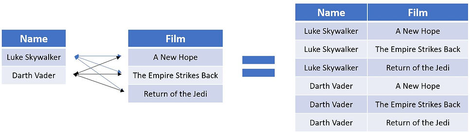
These types of joins are helpful if you ever need to compare all rows from one table against all other rows from a second table. This is done in the Yule's Q example where we need all product combinations. For this example I've gone a bit rogue and created a bespoke query to show how a tables of two character names can be paired up against a table of film names that we know hey starred in. The illustration of how the records merge also shows why the query is called a cross join.
Tips and Tricks
The next section just runs through some examples of challenges that can drop up when joining data out in the wild and some with some hints and tips on how to overcome them.
What if my tables have names in common but I'm not joining on them?
We saw earlier that SQL can't really handle column names that are common across table but not in 'on '. Instead we need to explicitly rename the duplicate column name in our SELECT statement with a new alias. In the code below a subquery creates a new column called 'species' to mimic the name in the humans data set even though they record different data. We can still bring both column into our final table after the join by renaming our second species column in our SELECT:
What if my join keys have different names in each table?
This is actually something SQL excels at and we don't need to worry about renaming columns before joining on them like we might in other languages. We simply tell SQL what the join columns are in the ON the same as normal. This time the subquery code changes the name from 'name' to 'character_name' to force there to be a mismatch in the join key name between tables. However all we do is tell SQL the the table aliases and column names we want to use in the ON:
What if I need to join on more than one column at a time?
So far all our joins have just been joining on one column at a time. Sometimes, particularly if we've got aggregated data, we might need to use multiple columns in our joins. This is again no problem for SQL, we simply pass it all off the columns in the ON. In the below example we join on 'name' and 'homeworld' even though in this instance iit doesn't affect what the final table looks like:
What if I need to join on multiple columns and they have different names?
If we've got multiple columns we need to join on and they've got different names we can combine the two previous approaches. We pass all of the relevant columns and their table aliases to the ON:
What if I want to join more than two tables at a time?
So far we've just been joining two table at a time. What happens if we want to add some more? The actual code to do this is nearly exactly the same as what we've been using. The important conceptual difference is that after our first join the 'left table / right right' changes when we come to our second join. When you have multiple joins, the concept of "left" and "right" table applies relative to each specific JOIN operation in the sequence. Essentially what this means is that once our first join has been specified, the result of that is now the left table that our next join anchors to.The "left table" for any given JOIN is always the cumulative result of all table operations that came before it in the query. The "right table" is the one being introduced by that specific JOIN keyword.
If that sounds a bit confusing here's a step by step summary of what happens in the below query:
-
We start with all of starwars_data.
-
We LEFT JOIN it with humans_droids based on matching names. If a starwars_data row has no matching humans_droids name, its humans_droids-specific fields (like b.homeworld) become NULL, but the row itself is kept at this stage.
-
Then, this dataset is filtered with the next INNER JOIN. Only those rows where the original starwars_data.name also exists in the humans table are kept for the final output. Any starwars_data entry that doesn't have a corresponding name in the humans table will be completely excluded from the final result, regardless of whether it found a match in humans_droids.
Filtering and joins: semi-joins and anti-join
So far we've looked at joins, some of which will occasionally cause us to filter out rows but really we've been interested in joining so we can bring in additional columns from the extra table. Now we'll look at a few instances of how we can use joins for the explicit purpose of filtering our data rather than to bring in new columns. We'll also look at some other handy filtering methods that use information from across different tables but might not join to them directly.
First up we'll look at what's called a semi join. A semi join is a type of join between two tables that returns rows from the first (or left) table where one or more matches are found in the second (or right) table. Unlike an INNER JOIN which can return columns from both tables, a semi join only returns columns from the left table. It uses the right table purely as a filter. Another difference is that if a row in the left table matches multiple rows in the right table, an INNER JOIN would return that left table row multiple times. A semi join, however, will return the row from the left table only once, regardless of how many matches it finds in the right table. We use a semi-join to filter for rows in the first table that also exist in the second table.
Unlike for our previous joins where there was specific syntax to tell SQL which joins to apply, for semi and anti-joins we instead create the logic ourselves. The below query tells SQL to SELECT all the data from humans_droids and then applies a filter with WHERE that uses the EXIST syntax to check for the existence of any matching row in the subquery i.e. the humans data set.


The second type of filtering join available is called the anti-join. Whereas the semi-join only returns rows that match in both tables, an anti-join returns rows from the left table that don't match rows in the right table based on our specified join condition. This can be helpful if say you've got a list of exclusions in one table that you need to apply to another. For example, let's say we've still got our sales by day table but we want to remove public holidays as we think these might skew our data. If we have a second table of public holiday dates we can anti-join against this to only keep dates in our first table that aren't in the public holiday table.
Like with the semi-join, SQL doesn't have a dedicated anti-join keyword. Instead, anti joins are typically implemented using LEFT JOIN with a WHERE IS NULL clause. The LEFT JOIN keeps all the rows in the first table and finds matching rows in the second. The WHERE IS NULL then SQL to filter to only return rows where there was no match i.e. rows that are in our left table and not in the right. Let's see how we can use it to remove all of the human characters from our 'humans_droids' data set. Note that as we're using a LEFT JOIN here if we have duplicates in our join key that match in both tables, this time we would get duplicate rows in our output table too.


Set operations: UNION ALL, UNION, INTERSECT and EXCEPT
So far we've joining tables side-by-side i.e. left and right. But what if we wanted to join top to bottom i.e. append new data to our table? This is where we can use our set operators UNION ALL, UNION, INTERSECT and EXCEPT. Since we're appending data these functions require us to have the same number of columns in the SELECT statement for each table. If one query selects three columns and another selects two, the operation will typically result in an error. We also need the columns to be in the same order in our SELECT statement. The operations combine the result sets vertically, column by column, based on their position in the SELECT list. If the order differs, data from one column might be incorrectly combined with data from a different column to the one we intended even if they're called the same thing.
Let's start with UNION ALL which, as the name suggests, keeps all the rows from our tables, even if they are duplicates of each other. As it doesn't worry about checking for duplicates it can be quicker than the UNION operator. We can UNION ALL are two table although we can only SELECT name as this is the only column shared across the tables. We'll sort by it to so we can see how the duplicates values appear.
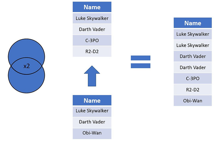
The new data set is 76 rows long which is a combination of 35 rows from 'humans' and 41 from 'humans_droids'. If we want to append data but without having any common rows occurring twice, then we can use the UNION join instead. It works in exactly the same way as UNION ALL except it removes any duplicate rows from the final data set.

This time we only get 41 rows of data as any duplicates have been removed. The last two set functions are INTERSECT and EXCEPT (sometimes called MINUS in some databases like Oracle). INTERSECT returns only the rows that are common to the result sets of all the SELECT statements involved. It effectively finds the 'intersection' of the datasets. INTERSECT also removes duplicate rows.


The EXCEPT function on the other hand returns distinct rows selected from the first table that are not found in the set of the second table.


That concludes this tutorial on joining data with SQL. You can see how these joins can be put to use in a project with this post on market basket analysis.