Machine learning in R with tidymodels

In this post you'll learn how to use the tidymodels package from RStudio to perform stratified sampling, pre-process your data ready for modelling, conduct resampling to get robust performance estimates and build regression and classification models using a range of different algorithms.

What is tidymodels?

Today's post is the first of two on tidymodels. Tidymodels is a collection of packages developed by RStudio that make modelling in R a lot easier by bringing the principles of the tidyverse to the modelling process. One of its main developers is Max Kuhn who created the caret package and if you're familiar with that you'll recognise some of he functionality in tidymodels.

"The tidymodels framework is a collection of packages for modeling and machine learning using tidyverse principles." - tidymodels.org

I've previously done a series of posts on caret (part 1, 2 and 3) and plan to follow a similar structure for this series on tidymodels. I try to keep these posts a mixture of theory as well as code but to avoid repeating myself too much this post will mostly be about working with and exploring the functionality of the tidymodels packages. To learn more about why some of the steps are necessary or a good idea you can refer back to the caret posts. The data exploration section in this post is pretty much entirely lifted from the first post in that series so if you're familiar with it feel free to skip that section. Otherwise I've included it here so today's post works as a stand-alone too.

The hope is that by the end of this tutorial you'll be able to build your own powerful and robust modelling pipelines utilising the full range of packages available in the tidymodels ecosystem. You can see a full list of the packages that come with tidymodels here and also some of the extra ones that don't come as part of the main package here. I'll try and flag which packages are used in each section. Topics we'll cover include:

Data splitting whilst preserving important distributions (stratified sampling) using the rsample package
Pre-processing our data with recipes in a way that avoids data leakage
Selecting a resampling scheme to get robust estimates of our model performance using rsample
Training and comparing different modelling algorithms with parsnip and yardstick
Calculating and understanding variable importance estimations and plotting the results with the vip package
Putting it all together into one seamless pipeline with the workflow and workflowsets packages

The next post will then build on these learnings and focus on how we can try and increase our model performance even more by covering:

Trying different 'engines' for our models from the parsnip package
Hyperparameter tuning using the dials, tune and finetune packages
Model stacking and ensembling using the stacks package

It's worth checking out the tidymodels website which is great and full of useful tutorials. There's also a tidymodels book from Max Kuhn and Julia Silge available for free online. Julia also posts lots of video tutorials using tidymodels.

An example tidymodels workflow

A lot of what we do in tidymodels is creating specifications for things (i.e. 'this is how X will be done') rather than doing the thing itself. The most obvious examples of this will be when we start using the recipes package to pre-process our data. This is helpful as it means everything is kept within our pipeline and then applied individually across each resample. For recipes for example, it means we avoid pre-processing our data too early and potentially leaking data between resamples. However, it does make it a bit harder to write a tutorial as you don't get to see a lot of the steps in action until the very end.

To that end, I've included an example tidymodels workflow below so you can get an idea of the different steps involved at each stage and how they all fit together. The other noticeable convention used by tidymodels is nested data. This allows for lots of complicated processing steps or output to be stored in single objects but again can be a bit confusing at first. The good news is that tidymodels makes heavy use of the broom package to 'tidy' the nested data and also comes with lots of helper functions to allow us to easily access and work with the parts that we want.

If you've done some modelling before, hopefully some of those steps look familiar in terms of how we split the data, specify what pre-processing we'd like and how we define our resampling scheme and then train our model. If it's completely unfamiliar don't worry as we'll go through each of the different steps in turn.

The diamonds data set

We'll be using the same data set throughout which is the diamonds data set from the dplyr package. We'll create some mock training data where we try to predict the price of the diamond based on its physical characteristics. Let's go ahead and load all the packages we'll need today. If we call the help function on 'diamonds' we can see that it is 'A dataset containing the prices and other attributes of almost 54,000 diamonds' as well as descriptions for each of the variables. We can have a quick look at the data by calling head() to print the first few rows and summary() to get a quick summary of each of the columns:

It looks like we've got a mix of continuous (carat, depth, table, price, x, y and z) and categorical (cut, color, clarity) data and also from our summary it looks like we've got some unrealistic values for some of our diamond sizes. Each of x, y and z are meant to record various diamond dimensions in mm so having values of 0mm should be impossible. Its likely that these values are in fact missing/unrecorded and have been defaulted to 0. We can correct this by replacing any 0mm dimensions with NA.

We also appear to have some very large diamonds which again could be indicative of some data entry errors. A quick bit of googling suggests the largest, clear diamond in the world, the Culinan 1, measures 5.89cm × 4.54cm × 2.77cm weighing in at 530 carats. So to get some diamonds in our data that are supposedly 5.89cm wide or 3.1cm deep suggests these are likely to be data entry problems. This becomes even more likely when we see that the largest diamond is supposedly only 5 carats and the most expensive is $18.8k.

It's worth mentioning that we're flagging and removing these outliers based on subject matter expertise to identify data entry issues i.e. incorrectly recorded data. This is different to identifying and removing outliers that are genuine data points but just larger/smaller/rarer compared to the rest of our data. It can be tempting to remove these kinds of outliers too but great care should be taken as outliers are data points too! There's a good discussion here about removing outliers. At the very least, removing outliers to try and improve our model counts as pre-processing our data and needs to be done as part of our wider model build and resampling scheme (more on this later).

For the sake of creating some extra missing data to use in this tutorial, let's pretend we know that one of our brokers occasionally uses the size measurements of the larger, uncut diamond by mistake. Therefore, any time we find a diamond with a physical dimension over 1cm or carat size over 3 we know it's a data entry issue and not to be trusted. We could remove these rows but assuming all the other the values (cut, color, etc) can be trusted we'll simply set them to NA and replace them with something more sensible later on.

As we'll be imputing (replacing the missing values with actual values) it can be good practice to create some new columns that record which rows had missing data. This can be particularly useful if we think the process that caused the data to be missing might be significant in our model. For example, the broker who entered the measurements from the uncut diamonds might also have recorded the price for the uncut stone which would generally be cheaper than an equivalent cut diamond. We'll see how we can do this easily with a recipe later on.

We can see now that we have a few missing values in our physical dimension features. As we'll be calculating feature importance estimates later on, let's add some random noise variables to our data to see if our model can correctly identify them as having no importance. We'll see during pre-processing how we can also remove variables that have little variation so let's add a column that is 99% populated with 0s too to demonstrate this:

Usually when building a model we'd want to do lots of feature engineering to try and create new variables for the model to use. As this tutorial is more about how to use the different tidymodels packages I'm skipping this step. Max Kuhn has also written an entire book on the subject that's available for free online. Now we've finishing mocking up our data, we can start using tidymodels to build our modelling workflow.

Splitting our data

We can split our data into Train and Test using the initial_split() function which creates a specification for splitting our data. We tell tidymodels which data set we want to use, the proportion of data to keep for our Training data and which column to use for any stratified sampling. Normally I'd take a 20% or 10% sample to be held out as a Test set and train the model on 80%-90% of the data. For the purpose of this tutorial I'm going to flip that and only have 10% of the data in Train. This is just to speed up the running of things as the data set is >50k rows. We'll still be training on ~5k rows of data which is enough to get a robust and predictive model at the end.

By telling tidymodels to use stratified sampling we preserve the distribution of the target column across both our Train and Test data sets. For example, if we had a categorical target where 50% of values were 'Yes' and 50% 'No', stratified sampling would make sure we'd have a 50:50 split between 'Yes' and 'No' in both Train and Test. For continuous targets like we're using, tidymodels converts our values into quartiles and then samples our chosen proportion from each group. This way we should end up with a matching distribution of our continuous target between Train and Test. Let's call our newly created object to see the print out:

It does indeed look like we've got 10% of our rows in the first split and the remaining 90% in the second. Note the naming convention of 'Analysis' and 'Assess' for our Train and Test splits. These follow the naming convention Max introduces in his book. The idea behind it is that although we have our Train and Test split, we usually also want to further split our Train data into folds or some other resampling scheme so we can measure model performance before we finally measure it on the Test set.

To avoid the confusion that can sometimes arise from referring to subsequent splits of Train as 'Train-Test splits' Max introduces the terms 'Analysis' for the data we train the model on and 'Assessment' for the data we measure performance on. How this typically works when we do our resampling is we have our initial Train and Test split and then the Training data is subsequently split into further Analysis and Assessment sets where we train and score our model, mimicking the Train-Test splits of assessing the model on unseen data.

To create our actual Train-Test splits from the specification we can use the training() and testing() functions and save the outputs into new objects. Let's go ahead and confirm that the stratified sampling worked correctly and that the distribution of price in both data sets is the same:

Those look pretty close! By design we can only pass one column to tidymodels to stratify on when sampling. If we think there are other important groups in our data that we want to preserve the distribution of there is a suggested workaround here where we create a new feature that is a concatenation of whatever fields we want to include.

It's worth noting that the more columns we sample across, particularly if some contain very small groups, the harder it might be to exactly preserve the underlying distribution of our original target column. In Max's response to the feature request in the link he also says this is something they purposefully didn't include as standard as often people try to stratify on groups where there simply isn't enough data in each class to make it possible which then causes things to error.

Let's create a mock version (which we won't use for modelling) of sampling across both 'price', which we'll manually bucket into quartiles, and also the 'cut' column:

Explore the data

We've already had a bit of a sneak peak at some of the distributions in our data when we were removing our data entry issues. Now we've split our data into Train and Test, let's have a more thorough look at how each of the different input variables are distributed. It's important to do this after splitting our data as the Test set is meant to represent unseen, new data and so we can't use it to draw conclusions about our data as a whole as in theory it doesn't exist within our workflow. I like to think of the Test set as representing tomorrow's future data that we'll have when come to deploy our model but doesn't exist today.

We can use the skim() function from the skimr package to get a very comprehensive overview of our data. This will help us understand what, if any, transformations we might might want to apply to our data further down the line:

From this we can see that nearly all the columns are complete and even those where we replaced the data errors with NA are still over 99% complete. Our price and size columns (x, y, z) all have tails of larger/more valuable diamonds. We can see this from the histograms and also from the fact that the mean value of the columns is higher than the median (p50). We can also see that our randomly generated variables do seem to be completely random. We can have a more thorough look at our data by creating some more detailed plots. First we'll split the numeric and categorical/binary columns off separately:

For our categorical columns, we're selecting anything that's not numeric and also our dummy 'low_var' flag column. For our continuous data, we're taking anything not in our categorical data and dropping the price column.

For categorical data, we can use box-plots to compare how the value of our target (price) varies for different categories within each of our columns. We can do this by creating a function that calls ggplot to create a box-plot and then pass the function to purrr to map over our vector of categorical columns:

There's quite a lot to take in with these plots! Firstly, it looks like there's something odd going on with the relationship between price and factors we'd normally think of as giving a good indicator as to the quality of the diamond. For example, the average value of a 'Fair' cut diamond is higher than one with an 'Ideal' cut. The same happens for colour. It looks like as the colour gets worse, the price goes up and the same for clarity too. We'll dig into this a bit more later on. For our randomly generated 'low_var' variable doesn't seem to show any great difference in average price which is to be expected.

Let's repeat the process for our continuous data by plotting a simple scatter plot. We can add a trend line to our plot to see what possible relationships there might be between our column and target and potentially flag any transformations we might need to do to our data:

Again we've got a lot of information in these charts. It looks like there's a strong, positive trend between price and carat which makes sense as we'd expect larger diamonds to cost more. The trend is pretty linear to start with but then flattens off when we get to the really big diamonds. For depth there's not a super obvious trend. Maybe for values from 55-60 it's weakly negative and then from 60-65 it's becomes slightly positive. Table is similar, looking like a positive trend between 55-60 but then flat after that. Variables where we don't have a clear linear trend or where we have a combination of different trends across different values of the same variable might mean linear models struggle with these and so we might want to try a different type of model to best capture the relationships contained within them.

The size in mm variables 'x', 'y' and 'z' all show very similar trends and all look similar to what we saw with carat. This makes sense as they measure the physical dimensions of the diamond which will then be captured by the carat/overall diamond size. Out of the three dimensions 'z' (actual depth in mm) looks to have the steepest curve suggesting diamonds become more costly per mm gained in depth than they do by getting wider. Finally, our last 4 noise variables show that they truly are random with a flat trend line amongst a random scattering of values.

Having seen the strength of the relationship between carat and price this might explain the strange trends we saw earlier with our categorical data. We'd expect bigger and better quality diamonds to cost more. We've seen that this holds in our data for larger diamonds but the better quality ones seemed to be cheaper which was odd. Could it be that size trumps quality when it comes to valuing diamonds? We can test this by replotting our categorical features and controlling in some way for diamond size. We'll create 4 buckets based on the carat variable and then replot our data for cut, colour and clarity within each of these groups. This will show us how price varies for different levels of our categorical features for diamonds that are a similar size:

These looked more like the trends we expected to see. The carat groups range from 1 (smallest diamonds) to 4 (largest) and we can see that for the smallest and largest carat groups, a better cut does seem associated with a higher price although it's less clear for the groups in the middle sizes. Likewise a better colour (D) seems to make for a more expensive diamond within each of the different carat sized groups. Possibly the most obvious trend is with clarity where there's a positive trend between price and clarity quality within each of the groups.

Now we've solved the mystery of our quality vs price plots is there anything we can do to help our model with the continuous data? Having seen the distribution of price from our skimr plot we know that most of our diamonds are at the cheaper end of the distribution but we do have a long tail of some more expensive ones. Often with distributions like this it can be helpful to take the log() of the variable to try and give a more normal looking distribution.

Although not quite a bell curve, our data now looks a lot more symmetrical which can be helpful to some of the algorithms we'll want to use. We can make a note to include a log transformation our the target in our recipe step later on.

What is tidymodels

Splitting our data

Explore the data

The diamonds data set

Example workflow

Checking for correlations

One-hot encoding

Checking for correlations between inputs

We've seen already that we've got a few different ways of measuring the size of the diamond in our data e.g. carat, x, y and z so it's reasonable to expect there to be a strong correlation between them. Some models can struggle with correlated inputs e.g. it can cause linear regression to have unstable coefficient estimates or reduce the estimated variable importance across the correlated features in a random forest.

We can use the cor() function from base R to check the correlations between our features. We need to make sure to pass it only the numeric features and also remove any NA values first:

We can see that, as expected, x, y and z all have very high correlations to carat. We might want to consider removing some of these as part of our pre-processing steps when we come to train our models.

Pre-processing and avoiding data leakage

Pre-processing our data correctly can have a big impact on our final model's performance. Some models are quite particular about how they like their data presented to them (the tidymodels team have a handy reference guide here). We might also want to try other transformation steps such as converting categorical data into numerical representations or replacing missing values.

What all these pre-processing steps have in common is that they run the risk of unintentionally leaking data, causing our model give us bias/overly optimistic performance estimates if they're not done properly. From the rsamples vignette: "It is critical that any complex preprocessing steps be contained inside of resampling so that the model performance estimates take into account the variability of these steps."

For example, let's consider what to do about the missing values in our data. Ideally we want to replace them with something sensible that our model can use. A simple way to do this would be to replace the missing data with the mean value of the column. However the precise value of the mean we use will depend on what data we have in our data set at the time. Remember that we take a separate Test set to replicate testing our model on new data i.e. we want to see how it performs on data not included in the model training process. However we also want a way of measuring performance across different models or data transformations before picking our final model.

The usual way to do this is to use resampling, either say using k-folds or bootstrapping, where each held out resample takes on the role of a mini test set. As we saw when we first split our data, to avoid the confusion of talking about test sets taken from Train, Max introduces the convention of Analysis and Assessment sets when talking about resampling. The resamples of Train that the model is built on are the Analysis set and the held out resamples for measurement the Assessment set. To get a robust measure of model performance when resampling we need to replicate testing our model on data that hasn't been in the training process otherwise we're leaking data from our Assessment set into our Analysis set. This means any pre-processing we do has to be done on the Analysis set only which means we can't just blanket apply any transformations to our whole Train data set. Below is an example of how a 5-fold cross validation resampling scheme looks:

One way to think of it is we can't do any pre-processing upstream on the Train as it's then impossible to separate this out further downstream in the resamples. To make it more obvious what's happening we can recolour our Train to reflect the fact it contains both Analysis and Assessment sets upstream and see how this affects calculating the average value we want to impute with:

The mean value for the whole of Train is 0.6 but we can see that actually the mean for our Analysis set is 0.55 and for our Assessment it's 0.8. If we'd used the 0.6 average value from Train for our imputations it'd be closer to the 0.8 of our Assessment and so our model would likely seem to perform better. However it's only appearing to perform better because we've inadvertently fed it information from the Assessment set which isn't going to be possible when we come to predict on the Test or future data. What we actually want to use for imputing missing values is the 0.55 from the Analysis set only. This might make the model performance appear worse but it gives us a more accurate measure of how we'd expect our model to perform on new data.

"In order for any resampling scheme to produce performance estimates that generalize to new data, it must contain all of the steps in the modelling process that could significantly affect the model’s effectiveness...preprocessing or filtering steps (such as PCA signal extraction, predictor correlation filters, feature selection methods) must be part of the resampling process"

- Feature Engineering and Selection: 3.4.7 What Should Be Included Inside of Resampling?

In his book Max also gives a few examples where you can bend these rules (e.g. imputing a few rows amongst many thousands or centring and scaling based just on the Train) and it's a judgement call if the chance/size of the bias introduced is acceptably small relative to the overall size of the data. For now though, we'll process our data in the formally correct way. Thankfully tidymodels and the recipes package make this really easy to do!

Pre-processing our data with recipes

The recipes package allows us to create sequences of feature engineering steps which we can combine using the dplyr pipe %>%. You can see here exactly how many different options (a lot!) we have for pre-processing our data. The order in which we specify the steps also determines in which order those transformations are applied. There's a handy guide here on which order to apply things generally works best. As mentioned previously, a lot of the steps in tidymodels create specifications of actions to perform rather than perform those actions outright.

In the case of recipes, we create the list of steps we want to perform on our data but they don't get run until we explicitly call them - either manually or as part of a wider workflow. This means, as well as being incredibly powerful and easy to use, we can seamlessly combine our recipe steps into our modelling workflow and resampling scheme. This ensures that each recipe step is applied within each resample during the model training so we avoid leaking any data and get unbiased estimates of our models performance.

To start a recipe, we simply call the recipe() function and pass in our model formula and data we want to use e.g. y = x1 + x2 or if we want to use all features we can just say: y = ~ . One thing that confused me initially when first learning about tidymodels was that often in tutorials, the data set passed to the recipe at this step was the entire Training data. Although this makes it look like the recipe will be applied to 100% of the Train data set, recipes only actually uses it to work out the specification for the recipe e.g. what variables will be in the data set, what format are they, etc. This is highlighted in the recipes with rsamples guide: "While the original data object...is used in the call, it is only used to define the variables and their characteristics so a single recipe is valid across all resampled versions of the data."

We can see from our simple recipe that it's identified 15 columns from our Training data with 1 given the role of outcome (price) and the other 14 the roles of predictors. Like any good recipe we can layer in more steps and adjust it to suit our needs. For example, we have the option to change the roles of variables. Say for example we have a row number or ID field in our data that we don't want passing to the final model. Rather than have to remove it, we can just use the recipe to a assign a non-modelling role i.e. not predictor and not outcome:

In the above example we add in a pretend row ID which we wouldn't want to pass to the model as an input. By default the non-outcome variables get set to a 'predictor' role but we can add an extra step to the recipe with update_role() where we tell tidymodels that the feature is actually something different. We can see from the print out that we now have 1 fewer predictor.

Another really handy feature of recipes is that we can select columns to apply different recipe steps to using dplyr-style helper functions e.g. 'starts_with()', 'all_numeric_predictors()', etc. For example, say we wanted to create dummy variables out of all our categorical predictors, normalise all of our numeric predictors and also perform a log transformation of our target column 'price'. We can easily create a recipe to do this for us:

We see in the print out that our recipe now shows we have added the creating dummies, normalising and log transforming steps and which variables are covered by each of them. What's not happened yet are any actual data transformations. We're still at the specification stage with our recipe and it's only when our recipe gets used as part of our modelling workflow that any pre-processing steps will be applied. Alternatively, if we want to apply our recipe outside of any modelling workflow, maybe to check the outputs or if we want to process our data in advance of training our model, we need to pass it a few extra steps, namely prep() and bake().

Applying recipes outside of workflows with prep() and bake()

Most of the time we'll probably be applying our recipes as part of our wider modelling workflow so we don't need to worry about prep() and bake() too much but it's good to know they exist. The prep() function tells tidymodels to calculate the parameters needed to apply the recipe steps and bake() applies those calculated parameters to our data i.e. it's at this point our data actually gets changed. When we're using recipes in a workflow the prep() is automatically done on the Analysis set in our resample scheme and then baked on the Analysis and Assessment set for us.

When we're calling prep() outside a workflow we can pass a specific data set to use for calculating the transformation parameters or we can leave it blank and it'll use the data set from the initial step in our recipe. As that first data set in the recipe formula is often our Train data, depending on what we're doing we need to make sure we don't accidentally pre-process our data in an incorrect way that leads to data leakage.

For example, if we're just baking our recipe to get an idea of how a transformation or pre-processing step behaves, but we're not actually overwriting any tables, then we can just prep() and bake() on Train. This is what we'll be doing in the sections devoted to exploring some of the different recipes steps available in more detail.

If however we're wanting to pre-process and save our data in advance of the model training then we need to prep() the data on a sample separate to Train. Otherwise we're calculating our pre-processing on 100% of Train again and so when we bake() it, we're leaking information across all of our resamples. We'll quickly cover how to prep and bake using a separate sample to avoid this but for our final models we'll be incorporating our recipes into our wider modelling workflow.

Prepping recipes on a separate sample

When we include our recipe as part of our workflow, any transformations have to be calculated per resample to avoid leaking data which can increase training time significantly. Another option if we have lots of data is to 'spend' some of it by taking a separate sample from Train that is purely used to estimate the data transformation parameters and then not used in the subsequent model build process.

As the transformation sample doesn't get used in the final build process we avoid leaking any data. The Train-minus-sample and Test both also get transformed using parameters from the sample data so we get a fair estimation of performance from the resamples on how our model should perform on the Test. Let's see how we could do this with our imputations in a way that applies prep() and bake() correctly:

In the above example we take a 20% sample from Train and use it to prep() our recipe. In this case we use a bagged tree model to impute any missing data. We then bake this recipe on train_80pct which is the Train data set minus the sample that was used to prep the recipe. This way instead of having to pre-process our data for every resample we just apply it all in one go. The sacrifice is that we use up a bit of our data to do so which means we have less to train our model on. Often whether we choose to apply our recipe this way or as part of a workflow will come down to how long it takes to run each version.

Now let's look at the other pre-processing options we have available to us in recipes. As we won't be saving any of the transformed data I'll just be use the Train data to prep() and bake() the recipes.

Imputing missing values

We've just seen the bagged tree imputation method and you can see a full list of all the imputation methods available in recipes here. I've included a selection below that can be roughly divided into two approaches. The first lot all use a model to work out what the missing values are likely to be based on information from the data set. These are likely to give a better guess at the missing value but potentially take longer to run. The second lot use a simple summary statistic e.g. mean, median, etc. or simply set missing categories to a new class of 'unknown'. These might yield a slightly cruder imputation but will be a lot quicker to run and maybe easier to explain to people.

In theory, something like the bagged tree model should be the most powerful when it comes to imputing our missing data but will probably take the longest to run. Potentially if we suspect our missing data might be in the tails of our distributions the linear model might do better or might offer a better trade off between performance and speed.

Let's try adding a bagged imputation model to our existing base recipe and then confirm that it does indeed replace all our missing values. We simply add the extra step with the %>% pipe and tell tidymodels which features we want to impute. This is already a huge improvement compared to what we saw with caret where if we use the imputation functions it calculates them for all columns which can make something bag impute unfeasibly slow. Let's go ahead and add the extra step to our base recipe and run it:

Transformations and Normalisation

As previously mentioned, some models prefer to have their data transformed e.g. normalised. The tidymodels team have a useful cheat sheet for which types of models benefit from different pre-processing steps and you can find a full list of available transformations here. Below is a list of some of the ones I use most often:

step_center() - normalises numeric data to have a mean of zero.
step_scale() - normalises numeric data to have a standard deviation of one.
step_normalize() - normalises numeric data to have a standard deviation of one and a mean of zero.
step_range() - scales numeric data to be within a specified range (uses between 0-1 by default)
step_BoxCox() - uses maximum likelihood estimation to estimate a transformation parameter to give the variable a normal shape (only works on values >0)
step_YeoJohnson() - like box cox but can handle negative and 0 values
step_log() - applies a log transformation to numeric data
step_ns() - creates new columns using natural splines - polynomial transformations of different parts of the original variable in such a way that the overall function is continuous.

The easiest way to see how these transform the data is to plot the before and after results of the transformations.

We can see our data ranges from just below 4 and up to 10 and looks to have two peaks. It also looks to have a long tail of higher values. Let's apply some transformations and see how they change things:

The step_center() and step_scale() haven't changed the shape of the data but the scales are different. The step_center() subtracts the column mean from each row and we can see that some values are now negative. The mean value of the column is now centred at 0 so we can see that our data is skewed to the right. The step_scale() also leaves the shape unchanged but again our scale changes. Scale divides each row by the standard deviation of the column. Often we'll want to apply both these transformations at the same time which is what step_normalize() does. The sklearn documentation has some great examples of why rescaling data can be so important.

By subtracting the mean and dividing by the standard deviation we ensure every column is on the same scale for our model to use. The chart on the left shows the output from centring and scaling where the mean=0 and each point is expressed in terms of the number of standard deviations it is away from the mean. Again the shape is unchanged. Another way to achieve a similar result is to simply rescale the range of values so they all sit between 0 and 1 which is what the step_range() transformation does on the right. Last up are our step_BoxCox(), step_YeoJohnson() and step_log() transformations which do change the shape of our data:

The new shapes the transformations create are very similar to each other as each transformation is trying to do something similar i.e. transform our data to be more 'normal' in shape. We can see our data does look more symmetrical now rather than having the long tail of higher values like before. Box-Cox tends to be quicker to run but can't handle negative or 0 values whereas Yeo-Johnson can. We can also see that the scales are slightly different between all three transformations.

As well as global transformations of features i.e. where the whole of the variable gets transformed in one go, we can also do piecewise transformations where we split our variable into chunks and then create new features to represent each chunk. An example of this which we'll see later might be to discretize or bin our variable into different groups in attempt to capture the different trends that might be going on within it. Binning generally means we lose information from our feature though.

Another option is to use splines to capture non-linear trends which we can do in tidymodels using the step_ns() function which stands for natural splines. Max has a section in his book about splines but essentially the process splits the variable into chunks and creates new features which are polynomial transformations (usually cubic) of that section of the feature. This allows for the modelling of non-linear trends by our models without having to apply a global transformation.

The advantage of this is if we have a very wiggly trend we might need a high powered polynomial transformation to capture it. The challenge with this is by increasing the power we increase the chances of overfitting our data and also that the transformation starts to oscillate in undesirable ways. Splines try to reduce this by fitting lower-degree polynomials (usually cubic so less wiggly) to individual sections i.e. they fit piecewise to try and capture the important trend in their section. Let's try running step_ns() on our 'depth' and 'table' features as from our plots they seemed to have the least linear trends. We can tell how many chunks to split our features into using the 'deg_free' option. Let's try with 3 degrees of freedom to start with:

We can see that we get 3 new columns per original feature. Splines are a great way to help linear models model non-linear trends. The more degrees of freedom we add the more complex trends our splines can capture but we run the risk of eventually overfitting our data. Another alternative is to pick a modelling algorithm that can handle non-linear trends by default and we'll see some examples of this later.

Dummy variables and target encodings

The recipes package also has lots of functionality for dealing with categorical or factor variables. Whilst some modelling algorithms in R are happy to accept factors as inputs (e.g. ranger and cubist) a lot of them require categorical data to be converted into a numerical representation. The simplest way of doing this is to create dummy variables or one-hot encode the categories but tidymodels also has some more advanced methods that are worth looking at. First up is the step_dummy() function which creates dummy variables out of of categorical columns:

Two things are immediately obvious here: 1) our dummy variable names are a bit unintuitive and 2) they're not dummy variables in the traditional sense of 0/1s. This is because our factors were ordered which if we look in the recipes documentation means: "For ordered factors, polynomial contrasts are used to encode the numeric values". If we want to avoid this and have some binary dummy variables we can use step_unorder():

These look more like what we were expected and have the added bonus that the names are clearer too. The downside with creating dummy variables is that we get as many new columns as we have levels in our factor. There is an option, 'one_hot=T', to tell tidymodels to make one fewer column than levels e.g. step_dummy(color, cut, clarity, one_hot = T) but we can still end up with lots of columns and for some of the less frequently occurring classes these columns will be mostly 0s. A way round this is to use the step_other() function to collapse rarely occuring levels of the factor into a catch-all 'other' level. By default it collapses any classes occurring less than 5% but we can up to this to 10% to demonstrate it:

We can see that each of our factors now has an 'other' column and that the total number of columns created has dropped from 15 to 12. As well as creating dummy variables from our factor columns we can also create some to record which rows and columns had missing data. This can be handy if we think that the cause of the missing data might be significant. For example, if we were trying to predict fraudulent claims at an insurance company, it could be useful to flag claims with lots of missing data as these might need to be treated more carefully. We can do this in tidymodels with the step_indicate_na() function:

Those look to have worked well. As well as dummy 0/1 encodings for categorical features, tidymodels has some more advanced methods available. These sit in a separate package called embed but we'll have a quick look at two of the methods for encoding categorical features and then later we'll see how it can bin/discretize our numerical features too.

Rather than just create 0/1 flags for our model to use, it'd be nice if we could also pass some meaningful information about the categories to our model at the same time. One way to do this is to replace the category with the average value of the target for each level in the category. We can do this using the step_lencode_glm() function which builds a linear model with no intercept for each level of the factor. As our target is continuous this means we get the average value of the target for each factor level.

The advantages of this approach are hopefully twofold. One is it should be more powerful than simply creating 0/1 flags to represent the different categories. The second is that it works well with categorical features that have lots of levels as we simply replace the levels in the original column rather than creating a new column per level. The potential downside is that as we're using known data about the target to pass information to the model, it can lead to the model overfitting. This is why it's so important to carry out our pre-processing on a separate sample or as part of our workflow.

We can confirm that what we've got are the average values of the target by comparing our recipe columns with the manually calculated average:

They're a match! We also saw earlier with the step_other() function that some of our factors had infrequently occurring levels. We might feel less certain about including the average target value for a factor level when it only has a few rows of data. One way round this to use 'partial pooling' where for factor levels with fewer observations, their averages are moved closer to the overall mean in the data set. There's an example using this technique in the tidymodels book. Let's have a go at applying it to our data using the step_lencode_mixed() function:

Let's compare the values from the partial pooling vs the actual average per level.

We can see now that we have some small differences between the encoded target mean and the actual.

Binning or discretizing numerical features

I'm not going to spend too much time on binning as it isn't something you generally want to do other than maybe when there are known significant cut-off points in your data e.g. water boils at 100 degrees Celsius, different income thresholds for different tax rates or age as determining things like entitlement to social security benefits. Max even has a section of his book called 'Discretize Predictors as a Last Resort'.

Essentially the worry is by going for bins we lose some information about the trend/distribution of our continuous data and also we run the risk of picking cut-offs for each of our bins that don't work well on new data. That said, tidymodels has cut a couple of approaches for binning/discretising data we can run through. The first is an unsupervised approach, step_discretize(), that simply buckets our data into equally sized (from a number of rows point of view) groups:

There are also two supervised methods for binning variables that are available via the embed package. The methods are supervised as they look at the distribution of the target to help decide what bins to use for the continuous variable. As such they can lead to overfitting i.e. the bins picked work really well on the Training data but fail to generalise so well on the Test data. The first approach, step_discretize_cart(), uses a decision tree and the second, step_discretize_xgb(), uses an XgBoost model:

We can see that the xgboost model created a lot more categories than the CART model.

Filters for correlated or near-zero variance features

Tidymodels has a few different filter methods for removing columns that could cause issues for our models. We saw earlier how we have correlated features in our data which can be problematic for some models. We also have a simulated low variance feature that we created at the start. Low variance features are those where the vast majority of values belong to a single class or value and so the information they contain is likely to be relatively low. Zero-variance features are those where all the values are of the same class/value and so have no useful information. We can see how we can remove highly correlated and also zero/near-zero variance features as part of our recipe. First let's look at our correlated features. We can use step_corr() to do this:

By default the correlation filter removes any features that have >0.9 absolute correlation values. It tries to do it in such a way that the fewest columns are removed to make sure all the remaining columns have an absolute correlation < threshold. In our case it's removed 'x', 'y' and 'z' which we saw earlier all had correlations >0.9 with each other and with carat. We might decide that losing 3 of our main size metrics is too many and we'll see another approach later to removing multicollinearity using principal component analysis.

For removing zero and near zero variance features we can use step_nzv() which applies two tests to our features and if they fail both of them they are removed. The first tests to see if the feature is very imbalanced i.e. nearly all the rows have the same value. To test for imbalances, tidymodels looks at the ratio of occurrences between the most common class and the second most common class. This is called the frequency ratio and columns fail the test when their frequency ratio is >19.

The second test is the number of unique values in the column. By default, the test for the unique number of values is 10+ so columns with <10 unique values fail the test. Therefore any features with <10 unique values and a frequency ratio of >19 are deemed to be zero/near-zero variance and removed. Let's see how this works with our data:

As hoped our 'low_var' feature we created has been removed and all our other features have been retained. When combining step_nzv() with something like step_dummy() it's good to check how the two interact as dummy variables with values of 0/1 automatically fail the unique values test. In theory if we have a good frequency ratio of 1s to 0s they'll still pass the second test and be kept but for infrequently occurring classes they might fail and be removed. This might be desirable in some cases or we might want to use step_other() to bucket the infrequently occurring classes into a larger group.

Principal Component Analysis (PCA)

Principal component analysis (PCA) takes our initial features and replaces them with linear combinations of themselves that capture as much information as possible from the original data. The new principal components are also uncorrelated with each other which makes them handy for machine learning. They can capture and combine highly correlated and also lower variance features which saves us from having to remove them.

The same number of principal components are created as we have features in our data but the first component captures most of the variance in our data, the second component the second most and so on. This diminishing return of information means we can usually capture most of the information in our data with fewer principal components than we had features. As such principal component analysis is often referred to as a 'dimensionality reduction' (fewer features) technique.

The step_pca() function in tidymodels gives us two ways of specifying how many principal components we want to create. By default 5 principal components are returned but we can change this by passing 'num_comp = X' as an option where X is the number we want returned. Alternatively we can pass 'threshold = X' which is a value from 0-1 that returns the number of principal components needed to capture that percentage of the variability from the original features.

The downside to PCA is we lose some interpretability from our model as our features are a mix of lots of different features and have names like PCA1, PCA2, etc. We can get a rough idea of what each of our principal components is representing by looking at the correlations between our initial features and each of the new principal components. Since we don't have lots of features there's less need for us to run PCA but we can try it as a way of removing the correlated physical dimensions features as an alterative to just filtering them out. As PCA uses linear combinations of features our data needs to normalised first so we'll run step_normalize() first.

So it looks like we can reduce down our four physical dimension columns into one principal component and still capture 90%+ of the variability. That's pretty helpful considering we've also removed some multicollinearity from our features at the same time.

Defining resampling schemes with rsample

Once we've decided on our recipe steps for pre-processing our data we need to pick a resampling scheme for measuring our model performance. Tidymodels has a few different resampling schemes available via the rsample package. One thing worth mentioning is why do we do resampling?

The resampling itself doesn’t directly help improve the training of the final model as all the interim models trained on the resamples are discarded at the end of the process. The interim models might even have different coefficients or features selected to the final model. This is fine as during resampling what we’re measuring is less ‘how will this exact model with these exact parameters perform’ but rather ‘if I were to use this process to build a model, how is that model likely to perform when it sees new data’. This then allows us to pick between different models we’ve built e.g. different algorithms, different combinations of hyperparameters or feature sets.

The value of resampling is that it allows us to test our model workflow before we commit to running it on the Test set. We only try one, final model on the Test data as if we test more than one and pick the best we've started to optimise our model to the Test set and so lose the ability to get an unbiased estimate of its general performance. Let's have a look at some of the most commonly used resampling schemes available in tidymodels starting with bootstraps().

The bootstraps() function takes a random sample with replacement from our Training data to create a new Analysis set of the same size. Any data not included in the Analysis sample becomes our Assessment set. We can tell bootstraps() how many of these bootstrap samples we want to create (the default is 25) and also which column to stratify on when sampling:

If we call our created resamples object we can see that it's a nested tibble with 25 rows (one for each resample). We can see the size of our Analysis set is 5,393 for each resample which is indeed the size of our Train data set. We can also see that the Assessment set sizes vary between bootstraps e.g. 2,000 then 1,984, etc. This is because we use the left out data from the sample-with-replacement bootstrap process i.e. a row might get picked only once for the Analysis set on the way to the sample selecting 5,393 rows or it might get selected multiple times. Each time a row gets selected multiple times this means there will be some rows that aren't selected and these go into our Assessment set. As there's a degree of chance to whether the same row gets selected multiple times or not that's why the size of the Assessment set can vary between resamples.

Next up is probably the most popular resampling scheme which is k-fold cross-validation. For this, we randomly split our data into k-number of groups or "folds" which are roughly all the same size. We then create our Analysis set out of k-1 folds and use the left out fold as the Assessment set. This continues until each fold has had a turn at being the left out Assessment set. We can also choose to repeat the whole process multiple times by 'folding' our data in different places so that we get different Analysis and Assessment sets between runs.

With 10 folds repeated 5 times we get 50(!) resamples. We can call tidy() on our rsample object to see exactly which rows go into each resample:

We can see that the tidy() function unnests the table and allows to see exactly which rows are in each fold, what its role is (Analysis or Assessment) and how this changes across different repeats. Looking at row 1 in Repeat1 for example, it gets assigned to the Assessment set in Fold05 and so is in the Analysis set for the other nine folds. Whereas in Repeat2 it's now in the Assessment set as part of Fold03.

Next up is mc_cv() which stands for Monte Carlo cross-validation but is also sometimes called ‘leave group out cross validation’. We essentially a take a random sample of data (without replacement) for our Analysis set and then the rest forms the Assessment set. If we want we can repeat this process multiple times like we did with k-fold cross validation. This approach can be useful when you have really large data as it might be unfeasible to run lots of resamples.

As mentioned, Monte Carlo cross-validation can be helpful for when we have very large data. Conversley, leave-one-out cross-validation, loo_cv(), can be helpful when we have very small data. For leave-one-out cross-validation, all the rows but one are used as the Analysis set and the left out row is the Assessment set all by itself. This then repeats until every row has been an Assessment set. So we end up having as many resamples as there are rows in our data set (and building a model for each of them too).

Finally there's a version of k-fold cross-validation, group_vfold_cv(), that's designed to work well with grouped data or for any data where we might have repeated measures of the same observation. For example, say to generate our data we recorded the selling price of diamonds over a 5 year period. Now it's possible that the same diamonds might have been traded multiple times in that time period. We might still want to build a model to estimate diamond prices based on their physical characteristics but ideally we don't want to end up with the same diamond occurring in both our Analysis and Assessment sets as it would skew the measurement. Let's create some data to see how this might happen:

So now each diamond occurs in our data 5 times with only the price being different. I added an ID column so we can tell which diamonds are the same and a 5% per year price inflation to reflect what might be changing market conditions. If we trained a model on this data and happened to have the same diamond, just from different years, in our Analysis and Assessment sets we're essentially leaking information between the sets. A better approach would be to make sure the same diamond can only occur in either our Analysis or Assessment set and this is what group_vfold_cv() does. It splits our data into folds whilst making sure that the entire group (e.g. the same diamond occurring multiple times) all go into either the Analysis or Assessment but don't get split across them.

We can check this by looking at what rows are in the Analysis and Assessment sets for our first set of resamples:

It does indeed look like all of our ID 1 diamonds are in the Analysis set for the first resample and we can see that none of them are in the Assessment set.

Principal Component Analysis

Impute missing values

Avoid leakage

Filters

Transformations

Resampling and cross fold validation

Recipes

Prep and bake

Spending data

Binning

Models specs

Workflows

Training models

Model specifications with parsnip

Just like how we created specifications of how we'd like our pre-processing to be performed using recipes, we do the same for our models with the parsnip package. Parsnip can be thought of as the natural successor to caret (hence the name). They both aim to create a unified interface for working with lots of different modelling packages in R without having to learn all the idiosyncrasies of those underlying packages. It does this by abstracting the main elements of the model specification and aligning all the arguments from across the modelling packages.

For a parsnip model specifications we need just three things and we can technically get away with providing just the first two:

the type of model we want to use e.g. linear regression, random forest, etc.
the 'mode' of the model e.g. regression, classification, etc
what engine we want to use i.e. which modelling package do we want to use e.g. ranger, randomForest, etc.

Let's have a look at how this works in practice. To create a specification for a linear model all we need to do is:

Pretty simple right? We create the specification for the type of model we want by calling that model type. You can see a full list of all the models you can call here. We technically also only need to tell parsnip that we want to use that model type to perform a regression as each specification comes with a default engine selected for us. For models with hyperparameters, parsnip also picks some sensible default values for those too. To see which engines are available or have a look at what hyperparameters are available for each model specification, parsnip has incredibly comprehensive documentation that can be access via R's help function.

We can see that we've got a long list of available engines for our linear regression specification. For example, we could quite easily swap out our 'lm' for a 'glmnet' one. We also get details about the hyperparameter options that are available with some of the other engines.To see a full list of engines available for each model specification we can use show_engines() function:

To change our linear regression to use glmnet, we can add in an option to manually specify the engine. We can also specify any hyperparameters we want to use in the model too. We'll cover hyperparameter tuning in more detail in the next post so for now I'll just include some dummy ones:

Note the slightly generic names of 'penalty' and 'mixture' for the hyperparameters whereas if you're used to working with glmnet in other packages you'll have seen these called 'lambda' and 'alpha'. This is done on purpose in tidymodels to minimise the effort required to remember what each different algorithm calls each of these options. The aim is also give them a slightly more intuitive name e.g. if you're not familiar with the inner workings of glmnet, 'mixture' gives you a better idea of what the parameter controls than 'alpha' would.

Now we've created out model specification, let's see how we can combine it with our pre-processing specifications into a workflow and then finally train some models!

Putting it all together with workflows

Up until now we've mostly been making lots of specifications. Apart from a little bit of prepping and baking with recipes we've not actually changed any data nor trained any models. The benefit of this modular approach to model building, where each section has its own specification, is that it makes our process incredibly flexible. This then makes it very easy to test and iterate lots of different models and recipes to try and create the best model.

The final bit of prep work before we start training models is to join all of our recipes and model specifications together into a workflow. Workflows are essentially modelling pipelines but as dplyr already has the pipe %>% the term 'workflow' was picked instead. We can pass in our pre-processing recipe, add our model specification and then pass it to a fit() call to train our model for us. Later we'll see how we can then combine multiple workflows into workflowsets which allow us to test lots of different models and pre-processing recipes all in the same pipeline. Let's start with a simple recipe and combine it with our linear model specification.

After creating our recipe, we can start our workflow by calling the workflow() function and then tell tidymodels that we'd like to add a recipe object with add_recipe() and also our model spec with add_model(). We can see from the print out that our workflow records everything and we're now ready to train our model!

Training models

So we've made our recipe, created our model specification, decided on our resampling scheme and added everything to our workflow. Now we're finally in a position to a train a model! Training models in tidymodels is done with the fit() function or a variation of it depending on whether we're doing things like resampling or hyperparameter tuning. To give us a robust estimate of our model's performance, we'll use our k-fold cross-validation scheme that we created earlier. This means when we come to call fit(), we need to call the fit_resamples() version. To train our model we simply pass it our workflow and our resampling specification:

Congratulations you've just fit your first model using tidymodels! Before we have a look at the output let's compare how using a workflow simplifies our model training code vs declaring our recipe or model specifications directly. There's no need to run these as they're just a more code-intensive version of what we've just run:

The first example isn't too bad, we simply pass our recipe and model specification objects separately but the second example is a lot bulkier. It might be ok as a one off but if we wanted to try multiple model specs with different recipes, writing it all out each time could quickly take up a lot of room. Let's now have a look at the output our linear model:

From the print out we get a nested tibble of our modelling results which isn't super informative. Thankfully, tidymodels has a lot of helper functions for extracting everything we need to know from our model. We'll run through a couple of the most useful ones below:

The collect_metrics() function allows us to see how our model performed across the resamples. The .metric column tells us which assessment metric has been used and the 'mean' column is how our model performed on our Assessment sets. It's called 'mean' to make it obvious that the performance is the average score from across each of our resamples. The 'n' column tells us how many resamples were used to generate the mean. For us it's 50 as we had 10 folds x 5 repeats.

We can see that we've got an R Squared value of 0.97 which is very high. We don't have the mean absolute error (MAE) though which would be helpful as we've logged our target. On a logged scale the MAE (for lowish values of MAE) can roughly be interpreted as the mean absolute percentage error of the model. We'll see how we can add that in later.

The show_best() function is handy if we've run a model with lots of hyperparameters as we can see which one performed best. Note that we also get a warning that we've not passed it a metric by which to choose the best model so it defaults to RMSE. We'll see more of this function in the next post on hyperparameter tuning.

If it encounters an error or some other issues sometimes tidymodels will write something useful in the notes section of the output. This can be accessed with collect_notes() which for us is empty. Finally we can call collect_prediction() to access the predictions made from our interim models. We get an error as we didn't actually tell tidymodels to save these predictions. These can be handy if we want to plot how our model performed on the resample Assessment sets to get an idea of where it might be struggling. We can tell tidymodels to save these results by passing a control option when we train the model.

Let's now re-run our model but this time we'll tell it to calculate MAE and also we can add a control option that tells tidymodels to keep the resample predictions.

We can see our model has an estimated final performance of around 0.12 MAE which is pretty good i.e. we're ~12% out on average in our prediction of the diamond price. That's not bad for a first attempt. If we call our collect_predictions() now we can see how our models did on our Assessment sets during resampling:

Workflowsets

We can see our prediction in the '.pred' column and the actual value of our logged target 'price'. One thing to note here is that we get the results for every Assessment set from our resampling scheme which as ours had 5 repeats means we get 5x the size of our original data set. We'll see when we do hyperparameter tuning that we also get the results for every combination of hyperparameters too so this can create a lot of data. Let's plot our results and see how our model performed. We'll add in a filter step to only bring back the predictions for the best performing model even though for now we only have one:

That looks pretty good too and confirms that our model appears to be performing well. It looks like maybe for the more expensive diamonds our model is predicting values that are a bit too high. If we wanted to try and use this model for real we'd then be at risk of overpaying for more expensive stones which would be a worry. We can confirm this by adding in a mutate step to our plot code to plot the residuals too:

Final model fit, predicting on Test and variable importance

One big difference between tidymodels and caret is that when we do resampling, tidymodels doesn't train a final model for us until we tell it to. This makes sense as if we have lots of models to try with different recipes or hyperparameters we usually want to inspect how the model is performing on the resamples before selecting our final model to build on all of Train. What this also means though is that we don't have any feature importance scores available to us until we train our final model.

To create our final model on 100% of Train, we call the last_fit() function and pass it our original train/test split object. We simply pass it our workflow so it knows where to get its recipe and model spec from:

As we pass it the split object from the start of our code we get two processes for the price of one. We train/fit our selected model on 100% of Train and then it automatically scores up the Test set with the newly created, final model. We can then run our collect_metrics() on it to see how our model performed on the Test set:

Let's merge the output back onto our resampled performance measures to see how they compare. I've had to pipe an extra data.frame() on the end to convert the output to a data frame rather than a tibble so R doesn't show truncated values of our estimates:

Looks like our estimated and actual performance measure are pretty close. This means our pre-processing was done in a robust, non-leaky way and our resampling scheme was effective in giving us an unbiased and accurate measure of the model's likely performance on unseen data. Well done! We can plot the actuals vs predictions from our Test data too to see how our final model performed on the Test data:

On the whole it looks like our model is doing a good job at predicting diamond prices. It looks like it might be overestimating prices for the more expensive diamonds which could be a worry depending on how we're intending to use the model. We can try some different pre-processing steps or modelling algorithms to see if we can fix this. It might also be a symptom of only having taken 10% of the data for Train rather than 80-90% like normal.

Now we've got our final model fitted we can use it to calculate the variable importance scores for each of our features. These scores will be based off the transformed features after being pre-processed by our recipe. Tidymodels doesn't include a way to calculate feature importance directly but instead makes us of the vip() package which can extract a number of model-specific feature importance scores for us.

It's worth having a read of how the different scores are calculated between models. For example, for our linear model the absolute value of the t-statistics for each feature is used whereas for glmnet it's the absolute value of the coefficient which will in turn depend on the underlying scale of our data. To get the variable importance scores from our final model we use the extract_fit_parsnip() to get our final model as a parsnip object and then we can simply call vi() on it or to plot the results vip():

We can see from the scores and the plot that color_J is the most important. We can get a helpful 'Sign' column as well that uses the model coefficients to tell us whether the feature has a positive or negative impact on the target. A negative Sign for 'colour_J' makes sense as it would be the worst colour value in the data set and so would usually be indicative of lower quality diamonds.

'Carat' is the second most important variable which makes sense as we saw from our original plots that it was strongly related to price but it also has a negative sign. What's going on here? This is likely due to the presence of the other size dimension features i.e. 'x', 'y' and 'z' that we saw were all correlated with 'carat'. What can happen in these instances for linear regression models is it can cause the coefficient of the correlated terms to flip. This is why it's good to have an understanding of where the variable importance scores are coming from and what they're showing.

We might want to try a different recipe that deals with the correlated variables or maybe try a different modelling scheme that is less susceptible to correlated features. Before we do this though let's see how we can get our models to train faster by utilising parallel processing.

Speeding things up with parallel processing

Tidymodels has the ability to run elements of the model training process in parallel which can greatly speed up the time it takes to train our models. For example, we have 10 folds repeated 5x as part of our resampling scheme. Each fold is essentially its own, separate instance of training the model so there's nothing to stop us (in theory) having 10 instances each training their own model concurrently.

The downside with this is that we need to keep multiple copies of the data in memory and we’ll be utilising a lot more system resource to do so. I've found the process can also cause my RStudio session to be a bit more unstable so I tend to only use it when I know I've got something that will take a long time to run (see the post on feature selection in caret for example).

Let's have a go at running our model using parallel processing and compare how much time we can save. We'll use the tictoc package to do this. First we’ll run a check to see the maximum number of cores we have available to use. You generally don’t want to use all of them as you’ll need at least one for your operating system. In this example we’ll create 8 clusters and register them. This effectively means we have 8 copies of our project all now running at once. From here we just run our modelling workflow as normal. I'll run one with and one without parallel processing and we can compare the differences in times:

Using our 8 clusters and running the model in parallel reduced our training time from 84.3 seconds to 20.67 which is about 4x faster. We'll use this speed boost next when we create workflowsets to run lots of different models and recipes all at once. After we've finished our parallel processing we can deregister the clusters and tell R to go back to running things sequentially:

Build and compare multiple models with workflow sets

Up until now we’ve been running a basic linear regression but there are lots of models available to use. One of the challenges with caret was not only picking what type of model to use e.g. ‘a random forest’ but also which package or 'engine' e.g. 'ranger'. Tidymodels makes this a lot easier for us by packaging a default engine inside each model specification.

It even extends this to choosing sensible, default hyperparameters for a model when that model is the default engine. This means there's nothing stopping us from making use of this to create lots of model specifications with just a few lines of code:

Just like that we've got 14 different model specifications (15 if we include the glmnet spec we made earlier). We've got specifications for running everything from linear regressions and k-nearest neighbours to random forests, support vector machine and neural networks all created with just a simple function.

We've seen how we can easily combine recipes and model specifications into a workflow. When we've got lots of objects like this we can use a workflowset. These allow us to pass a list of recipe objects and a list of model specifications to create a large workflow set, which we can then run all in one go. Let's start with a fairly basic recipe and try running it with each of our models to establish a baseline for their performances. I like to give my recipes names that capture what they're doing to make it easier to see which type of pre-processing might have performed better:

To create our workflow set we call the workflow_set() function and pass a list of recipes to 'prepoc='. Although not strictly required, it's good practice to name each recipe in our list as the final ID for each recipe-model combination comes from the names and so can make identifying them easier later on. If we don't use names the ID will default to a generic 'recipe-<modelspec>-<rowID>' type name which can make it hard to tell the different models apart. As we only call each model type once (apart from lm and glmnet) I won't name them for now (apart from glmnet).

After our recipes, we then pass a list of all our model specifications (ideally named) to the 'models=' option. Finally at the end is the 'cross=T' which tells workflow set to do a cross-join between every recipe object and every model i.e. every model gets tried with every recipe. If we don't want to do a cross-join we need to pass each recipe per object ourselves so the lists are the same length.

From the output we can see we've got a tibble of 15 rows that contains all the information to run each of our models. We can run our entire workflow set by using the workflow_map() function. We simply pass it our workflow set name, the resampling scheme we want to use and whatever metrics we want to calculate. The 'verbose=T' option just has tidymodels print extra information about the run time and what step it's up to:

We can see the whole process took 378 seconds to run and there was quite a large range of run times between the different models from 12 to 44 seconds. We can also see that we got lots of messages about there being no tuning parameters. We'll see how we can add these into the process in the next post.

To access the results of our workflow set we can use the same collect_metrics() function that we did earlier:

This is helpful to see how the different models performed but it might be more useful to have them ranked for us. This is what the rank_results() function does:

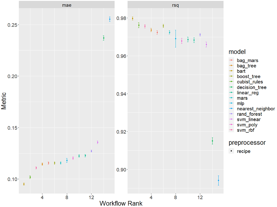
This is a bit more helpful. We can see that our top performing model was the BART model with a MAE of 0.095 and then the cubist model in a fairly close second with 10.2. Both models are the only ones to manage a MAE<0.011. We can see our standard linear model ranked 10th overall and our lasso implementation of glmnet came in at 12th. This suggests our data might have non-linear trends and possibly some important interactions that the tree-based and non-linear models that scored well can capture but our more linear models couldn't.

We can also easily compare our models in a more visual way too with the autoplot() function and this is where tidymodels being part of the tidyverse really starts to shine through:

Having established a benchmark performance for each of our model specifications we can now try and improve them a bit more by trying our models with some different recipe specs. Referring to the tidymodels pre-processing guide we can see that both the top models are actually incredibly robust with regards to the sorts of data they can accept. They can both handle factors and missing values natively and also don't massively benefit from transforming, normalising or reducing collinearity amongst the predictors. This might in part be why they performed so strongly to begin with. To demonstrate running multiple models with multiple recipes though, let's try a few variations of our original recipe:

We can then pass these to our workflow set as an extended version of our recipe list (making sure to name each one). This time rather than call every model we can just select the BART and cubist model as these performed the best last time:

Let's have a look and see how our models performed:

After all that it looks like leaving our data untransformed actually led to the best models for both BART and the cubist model! Although a bit of an anticlimax, it does make sense as both models are very flexible and robust in terms of how they can accept their data and it agrees with the tidymodels guide that there might not be much benefit to tinkering with the data before we pass it to the models.

Let's see how we can extract the best performing model from our workflow set and fit it to Train/Test to get the final measure of our model's performance. I'm actually going to use the cubist model as I got a bug where parsnip couldn't pull through the BART model. It at least allows me to demonstrate how to pick a different model from a workflow set rather than just the best one.

Remember for the last_fit() function we needed to pass it a workflow? To get that from our workflow set object we can run extract_workflow() and pass the function the workflow set and also the workflow ID of the model we want. We can type out the name of the workflow ID but I prefer to use the pull() function to create it automatically from our final model in the workflow set as it makes it easier to build automated pipelines:

That looks a good score on the Test set and it's very close to our resamples estimate which is good. Let's have a look at feature importance and plot the results of our predictions on the Test set.

These variable importance all look sensible and it's nice that the factor columns can be displayed in their original form too. The three size dimensions followed by clarity all make sense as being the most important factors. Let's now plot how the predictions of our final model did on the Test set:

tidymodels final model actuals on Test.PNG

That looks pretty good and it looks like it's doing a better job on the more expensive diamonds too which was a weakness with our linear regression model. Well done!

Classification models with tidymodels

So far all of the examples have been about regression but we can reuse a lot of the same steps to easily build a classification model. Let’s very quickly fudge our data to create a mock classification problem to demonstrate this. If we have a quick look at our original data again we can see that the top 25% of diamonds have a price of $5,324+.

Let's create a new target called 'expensive' which will represent these high value diamonds. For classification problems like this we can encode the target as a factor. The levels don't matter so we'll go with a “Yes/No” factor for our target column. After that we can recreate our split object, redo our samples and create our default model specifications but this time with 'mode = classification'. We can tweak our recipe to tell tidymodels not to use the price column and then we can put it all together in a workflow set just like we did before:

Hopefully all the steps above are familiar from working through the regression problem and we can see that we've once again got a good selection of strongly performing models. With ROCs that high it looks like it wasn't much of a challenge predicting expensive diamonds but we can see that our Test set and resamples score at least match so our model was genuinely doing a good job rather than overfitting.

Next steps: hyperparameter tuning and model stacking

In this tutorial we've covered splitting and transforming our data as well as running a few different 'out the box' (untuned) models. We've seen how to pre-process our data in a way that avoids leaking information, combine different models and recipes and assess their performance and also how tidymodels can be used to easily move between building regression and classification models.

In the next tutorial we'll see how we can try and improve our model's performance even more by tuning hyperparameters and also creating 'super learners' by stacking/ensembling different models together.

Speeding things up with parallel processing

Classification models

Hyperparameter tuning and model stacking

Feature importance

Machine learning in R with tidymodels

In this post you'll learn how to use the tidymodels package from RStudio to perform stratified sampling, pre-process your data ready for modelling, conduct resampling to get robust performance estimates and build regression and classification models using a range of different algorithms.

Contents

What is tidymodels?

"The tidymodels framework is a collection of packages for modeling and machine learning using tidyverse principles." - tidymodels.org

An example tidymodels workflow

The diamonds data set

Splitting our data

Explore the data

Checking for correlations between inputs

Pre-processing and avoiding data leakage

Pre-processing our data with recipes

Applying recipes outside of workflows with prep() and bake()

Prepping recipes on a separate sample

Imputing missing values

Transformations and Normalisation

Dummy variables and target encodings

Binning or discretizing numerical features

Filters for correlated or near-zero variance features

Principal Component Analysis (PCA)

Defining resampling schemes with rsample

Model specifications with parsnip

Putting it all together with workflows

Training models

Final model fit, predicting on Test and variable importance

Speeding things up with parallel processing

Build and compare multiple models with workflow sets

Next steps: hyperparameter tuning and model stacking

Copyright © 2024 Step by step data science. All Rights Reserved

Machine learning in R with tidymodels

In this post you'll learn how to use the tidymodels package from RStudio to perform stratified sampling, pre-process your data ready for modelling, conduct resampling to get robust performance estimates and build regression and classification models using a range of different algorithms.

Contents

​

What is tidymodels?

"The tidymodels framework is a collection of packages for modeling and machine learning using tidyverse principles." - tidymodels.org

An example tidymodels workflow

The diamonds data set

Splitting our data

Explore the data

Checking for correlations between inputs

Pre-processing and avoiding data leakage

Pre-processing our data with recipes

Applying recipes outside of workflows with prep() and bake()

Prepping recipes on a separate sample

Imputing missing values

Transformations and Normalisation

Dummy variables and target encodings

Binning or discretizing numerical features

Filters for correlated or near-zero variance features

Principal Component Analysis (PCA)

Defining resampling schemes with rsample

Model specifications with parsnip

Putting it all together with workflows

Training models

Final model fit, predicting on Test and variable importance

Speeding things up with parallel processing

Build and compare multiple models with workflow sets

Next steps: hyperparameter tuning and model stacking