Scikit-learn tutorial for machine learning in Python

In this post you'll learn how to use the scikit-learn package to perform feature selection and hyperparameter tuning to try and improve our base model's performance. Then we'll cover how to ensemble and stack different models into a super-learner before finally using shapley values to understand the contribution of individual features in our final model.

Introduction and prepping our data
Feature Selection
- VarianceThreshold
- SelectKBest
- RFE (Recursive Feature Elimination)
- RFECV (Recursive Feature Elimination with Cross-Validation)
- SelectFromModel
- SequentialFeatureSelector
Hyperparameter tuning
- GridSearchCV
- RandomizedSearchCV
- HalvingRandomSearchCV
- Optuna (Bayesian optimization)
Model stacking and ensembles
Understanding predictions with SHAP

Introduction and prepping our data

Welcome back! In the first part of this tutorial, we saw how to use scikit-learn to build a complete modelling pipeline from start to finish. We took the raw diamonds data, created training and test sets, built several pre-processing pipelines and compared over 20 different modelling algorithms to find the best performers.

So far, we've run our models with their default settings and used all the available features. In this post, we'll explore three techniques to try and improve our models' performances even more.

Feature Selection: We'll learn how to automatically weed out uninformative features to reduce noise and potentially speed up training.
Hyperparameter Tuning: We'll go beyond the default settings and see how to systematically search for the optimal parameters for our models.
Model Stacking: We'll learn how to combine the predictions of multiple different models into a single, more powerful "super learner".

At the end we'll also spend a bit of time looking into 'Explainable AI' by using the SHAP library to look inside our final model and understand why it makes the predictions it does.

The first tutorial aimed to cover cover everything you need for building and comparing robust modelling pipelines in sklearn. This one covers some more advanced topics to try and help squeeze out some extra performance from your model. Typically you're more likely to see bigger performance gains from better from better data, feature engineering and picking the correct algorithm for your data than you are from excessive feature selection or hyperparameter tuning. A lot of the best modern models like LightGBM and Cat Boost have in-built feature selections and sensible starting parameters out of the box. Nevertheless, it's good to have an idea of the different techniques available so let's go ahead an import our packages.

As you can see that's a lot of sklearn functions we'll be covering! For now, let's read in our data again and create the functions and pipelines from the previous tutorial that we'll be reusing in this one.

So we've got our diamonds data split into 10% train (to make things quicker to run) and 90% test. We've created our 5-fold cross validation schema and added a couple of useless, random noise features to our data and one that is mostly 0s. We've defined objects to store our numerical and categorical features and created a couple of pipelines that performed best from the previous tutorial. The base_pipeline is our CatBoost model that performed the best out of everything we tried last time. Before we jump into feature selection let's run our baseline model again to see how it performs.

The CatBoost pipeline is already a bit complicated with the pre-processing steps and the target transformer. However we'll see how we can pretty easily incorporate feature selection, hyperparameter tuning and model stacking into it. If you want to try this code with your own model or you don't want to have to worry about transforming the target, you can mostly just replace that section with something simpler in the pipeline like in the example below.

Now we've got our data and pipelines prepped and ready to go, including the addition of some useless variables, let's explore some of the techniques that we cam use to try and identify and remove these.

Feature Selection (and how not to do it)

Not all features are created equal. Some are highly predictive, while others might be redundant or just random noise (like the ones we deliberately created!). Feature selection is the process of automatically selecting the most relevant features for your model. This can lead to simpler models that are easier to interpret, faster training times and reduced overfitting by removing irrelevant noise.

Max Kuhn has chapter called 'Effect of Irrelevant Features' in his book 'Feature Engineering and Selection: A Practical Approach for Predictive Models' that shows that even models with built-in feature selection can suffer a drop in performance as the number of uninformative predictors increases. However in this video he also states that whilst feature selection methods work, they are so computationally intensive that it's not always obvious they're worth the extra cost.

Scikit-learn offers several strategies for feature selection, which we'll explore below but before we look at the different methods, it's crucial to understand how not to do feature selection. Performing supervised feature selection (i.e. selecting features based on how they relate to our target variable) is akin to training a model on our data and if we're not careful is a sure-fire way to introduce data leakage.

For example, let's say we calculate the correlation between all our features and the target and then only keep the highly correlated ones. If we do this, we're using information from the target variable to pick the best features but then using that same data to evaluate the model's performance. Unsurprisingly, the model will probably appear to do a great job. Even if we use a cross-validation framework for our model evaluation, the results are still biased because the feature selection was done upstream. We introduce data leakage because we ran our feature selection on the entire training dataset before resampling.

The correct way to perform supervised feature selection is to include it inside your cross-validation loop. This way, for each fold, the feature selection is performed only on the analysis portion of the data, and the performance is validated on a hold-out set that it has never seen. Thankfully, scikit-learn pipelines make this easy to do correctly as we'll see. To start with, we'll just look at how the different feature selection techniques work in isolation just to have some working example before running them as part of a proper pipeline later on.

Removing Low Variance Features

The simplest form of feature selection is removing features that have little to no variance. A feature that is the same (or almost the same) for all observations is unlikely to have much predictive power. We can use the VarianceThreshold transformer for this. In simple terms, it measures how spread out the data points are from their average value (μ). A variance of 0 means all the values in that feature are identical. Let's see if it can correctly identify and remove the 'low_var' feature we created, which is 0 for 99% of its values.

We can see that 'low_var' was successfully removed while all the original features (as well as our random ones) were kept. This highlights another important aspect of the VarianceThreshold transformer, it is actually an unsupervised method i.e. it doesn't consider the target variable when deciding to remove the feature. The features aren't removed because they have a uninformative relationship with the target but rather because their own inherent properties (low variance) which we're assuming would make them unreleated to the target (although this might not always be the case).

We can easily add VarianceThreshold to a pipeline because it works just like any other pre-processing step, such as an imputer or a scaler. It takes the data from the previous step, transforms it by removing low-variance features, and then passes the remaining features to the next step. In the below code, the pipeline is pretty much identical to our original base_pipeline except we've inserted VarianceThreshold after our pre-processing step (imp_ordinal) and before the final model. Let's compare the performance of our CatBoost model on the original feature set and on the feature set after the VarianceThreshold has been applied.

Nice! From the output it doesn't look like removing the feature has made much different to CatBoosts's performance.

Although we already know which feature gets dropped, let's see how we can extract the final variables from our more complicated pipeline. First, the entire pipeline is trained on the training data. During this process, each step is fitted. The VarianceThreshold step calculates the variance of every feature it receives from the preceding columntransformer step. After fitting, we can access the individual steps of the pipeline using .named_steps.

var_thresh_pipeline.named_steps['variancethreshold'] retrieves the fitted VarianceThreshold object.
The .get_support() method then returns a boolean mask—an array of True and False values. Each value corresponds to a feature: True means the feature's variance was above the threshold and it was kept, while False means it was removed.

To know which feature each True or False value corresponds to, we need the feature names. Since VarianceThreshold comes after the pre-processing step (columntransformer), we ask the columntransformer for the names of the features it passed along.

Univariate Feature Selection

In contrast to the unsupervised method, univariate selection methods examine each feature individually and measure the strength of its relationship with the target variable. We can then select a certain number of the "best" features based on these statistical scores.Univariate Feature Selection is a quick and simple method for reducing the number of features by evaluating each one independently against the target variable using statistical tests. This is a two-step process:

Score each feature using a statistical test (e.g., f_regression or mutual_info_regression).
Select features based on these scores (e.g., SelectKBest to get the top k features, or SelectPercentile to get the top n% of features).

The main pros of Univariate Feature Selection are generally its speed and simplicity.

Speed and Efficiency: Because it assesses each feature in isolation, this method is computationally very fast and requires less memory. This makes it an excellent choice for an initial filtering step on datasets with a very high number of features (e.g., thousands or more).
Simplicity and Interpretability: The techniques are easy to understand and implement. Statistical scores like F-values or chi-squared stats provide a clear, model-agnostic ranking of how strongly each individual feature is related to the target variable

The main downside of it are that it:

Ignores Feature Interactions: This is the most significant drawback. Univariate selection cannot detect features that are only useful when combined with others. For example, a feature might have a low individual score but be highly predictive when interacting with another feature. By ignoring these multivariate relationships, it risks discarding valuable information.
Disconnected from the Model: The selection is based on general statistical tests, not on what a specific machine learning algorithm might find useful. A complex, non-linear model (like a Gradient Boosting Tree or a Neural Network) might be able to extract predictive power from a feature that a simple statistical test deems unimportant.
Risk of Errors: By looking at features one by one, the method is prone to making mistakes. It might discard a feature that is part of a complex, non-linear relationship or keep redundant features that are highly correlated with each other, as it doesn't consider the context of other selected features.
The Impact of Correlated Features: the statistical tests (f_regression / mutual_info_regression) assume features are independent. Highly correlated features can distort results.

Let's try selecting the 8 best features using two different scoring methods. Note that these selectors can't handle missing data, so we'll need to impute our numeric features first.

It looks like both techniques have kept the original features and then had a slight disagreement about which of our dummy features should be included. Let try running f_regression with 8 features in our pipeline and see how it preforms.

Again, we've not got a huge change in performance. Let's extract the features that made it into our model in a similar way as before.

Recursive Feature Elimination (RFE)

Recursive Feature Elimination (RFE) is a powerful 'wrapper method' for feature selection. It "wraps" the feature selection process around a model, using the model's performance or feature importances to decide which features to keep. Max Kuhn has a chapter on RFE in his book here. It works by:

Building a model on all features.
Calculating an importance score for each feature.
Removing the least important feature(s).
Repeating this process until a desired number of features is left.

RFE is powerful because it considers the relationship between features and is tied directly to a model's performance. One weakness is that it is a so-called "greedy" search method. Once a feature is removed, it's gone forever and is never re-evaluated. This can sometimes lead to a sub-optimal final set of features. The main downside of the approach however is that the process of repeatedly building and evaluating models on different subsets of features iteratively also makes it very computationally expensive and slow.

Let's try running RFE on our data. One of the challenges for the standard RFE implementation is that we have to tell it in advance how many features we want it to select in the final iteration. Let's ask for 5 and see how it does. We also need to tell it what model to use in the iterative process. This needs to be a model that has some form of inherent feature importance baked into it e.g. the coefficients of a linear regression or the feature importance from a tree based model. For this example let's use a simple RandomForestRegressor as it's quick to run.

We can see that from the output that the the random forest has done a pretty good job of weeding out the known low variance and random noise features first. We'd asked for 5 features to be kept which means one of the original features had to miss out. Reassuringly, it looks like the original feature 'table' got removed last i.e. after the features we know to be less useful than it. Recursive Feature Elimination is a powerful tool, but its effectiveness depends heavily on how we use it. Simply running it with default settings might not give the best results. In general, there are two rules of thumb we can use to try to get the most out of it.

Firstly, the model we choose as the estimator inside RFE should ideally come from the same "family" as our final model. Different models find different kinds of patterns important. Linear Models (like LinearRegression, Lasso) rank features based on the magnitude of their coefficients, which captures linear relationships with the target. Tree-Based Models (like DecisionTreeRegressor, RandomForestRegressor) capture non-linear relationships and interactions and rank features based on how much they reduce impurity (Gini impurity, entropy) when they're used to split the data. If we use a linear model for RFE for example to select features for a final tree-based model, we might accidentally discard features that have a strong non-linear relationship with the target. By keeping the model families consistent, we ensure the features being selected are the ones most likely to be useful for your final model.

The second thing to bear in mind is that the model we use inside RFE needs to be treated like any other model, and that means applying the correct pre-processing steps to its input data. This is especially critical for linear models. They use the size of the feature coefficients to determine importance but the coefficients are highly sensitive to the scale of the features. A feature with a large scale (e.g., values from 10,000 to 100,000) will naturally have a smaller coefficient than an equally important feature with a small scale (e.g., values from 0 to 1). However if we don't standardise our feature in some way when we run our RFE model the larger scaled feature will also end up looking less important due to its scale alone.

Let's demonstrate this with a simple example. We'll create a dataset with two features, 'a' and 'b', and use RFE with a LinearRegression model to select the single best feature. The first bit of code just makes a dummy data set of 200 observations with 2 informative/useful features for the classification problem.

Using RFE with a linear regression, we can ask for 1 feature which means the model has to run for two iterations and gives us the ranking of which of the two features it found most important. As it's a linear regression, the importance comes from the size of the coefficient. Initially, with the features on a similar scale, RFE ranks feature 'a' as more important.

What happens then if we decrease the scale of 'b' and re-run the analysis?

Suddenly, RFE thinks 'b' is the most important feature! It has been fooled by the change in scale. The model had to give 'b' a much larger coefficient to compensate for its smaller values and RFE misinterpreted this large coefficient as high importance. To avoid introducing issues like this into our pipeline we can pre-process our data for the RFE model like we would for any other model. In this case we can simply scale our data before RFE. When we apply a StandardScaler, it puts all features on a level playing field.

By scaling the data, RFE can now accurately assess the true contribution of each feature, regardless of its original scale and feature 'a' is back being the most important. Scaling features is less of an issue for tree-based models but these can have their own challenges when calculating feature importance. Lots of highly correlated features in a tree based model can cause the important for each of them to be lower and high cardinality features (categorical feature with lots of different values) can artificially get high importance scores too.

In terms of incporporating RFE into our pipelines, whereas before with something like SelectKBest, where it's a standard pre-processing transformer, RFE is a meta-estimator that wraps and repeatedly uses another model. This creates differences in how the feature selection step is structured in our pipeline and how we interact with it. Let's quickly run through the main differences this causes.

Methods such as the SelectKBest object behaves just like other pre-processing tools, such as StandardScaler or SimpleImputer. It's a simple, self-contained step. We pass it its own parameters directly (e.g. for SelectKBest this was the scoring function f_regression and the number of features to keep k=8). It doesn't need a separate model to function. When .fit() was called on the pipeline, SelectKBest received the data from our imp_ordinal step and the target variable y. It ran its statistical test once to calculate scores for each feature and determines which ones to keep. After fitting, we can get the results directly from the SelectKBest object. The most common method is .get_support() to get a boolean mask (True/False) of the selected features. We can also access the .scores_ of each feature.

RFE is a meta-estimator, meaning its primary job is to control another model. This makes the construction more complex because its main parameter is the estimator—an entire machine learning model that will be used to judge feature importance. We're effectively nesting an entire model inside this pipeline step. This also introduces extra parameters like importance_getter, which we must use to tell RFE how to find the feature importances within its nested estimator.

When .fit() is called, RFE doesn't just perform a single calculation. It goes through an iterative process of fitting its internal estimator multiple times, removing the least important features at each step until only the desired number remains. This is a much more computationally intensive process than SelectKBest. The information it stores is also richer. While it also has a .support_ attribute (the final boolean mask), its most useful attribute is .ranking_, which tells us the elimination order of all features. A rank of 1 means the feature was selected, 2 means it was the last to be eliminated and so on. We can also access the final fitted internal estimator via the .estimator_ attribute.

If all of that sounds complicated, don't worry! Let's see it in action in a pipeline to hopefully bring things to life a bit more.

There are a couple of important details here. Notice the estimator we've passed to RFE is not just a RandomForestRegressor. Because our entire workflow transforms the target variable (using TransformedTargetRegressor), the model used inside RFE also needs this transformation to accurately assess feature importance. We therefore pass it a TransformedTargetRegressor that wraps the random forest.

The 'importance_getter' argument is a crucial and slightly tricky parameter. RFE needs to know how to get the importance scores from its estimator. For a simple estimator like RandomForestRegressor, it would automatically look for an attribute named .feature_importances_. However, our estimator is now a TransformedTargetRegressor. The actual random forest model is now nested inside it, at an attribute called regressor_. Therefore, the feature importances are located at regressor_.feature_importances_. We have to explicitly tell RFE this path using importance_getter = "regressor_.feature_importances_". For a linear model, this would typically be "regressor_.coef_".

Based on these results, the Recursive Feature Elimination (RFE) looks like it actually performed worse than our other methods. Maybe asking for 10 features was too many since it got outperformed by the SelectKBest which only kept 5. Let's see which features it picked for the final model.

RFE with Cross-Validation (RFECV)

One of the challenges with RFE is that we have to tell it how many features to select in advance. Should it be 10, 8, or 5? This is often just a guess. Thankfully, scikit-learn provides RFECV, an extension that automatically finds the optimal number of features for us. It performs RFE within a cross-validation loop (hence the "CV") to identify the number of features that produces the best, most generalisable model performance. This data-driven approach is far more robust and is generally the preferred method. There's a nice example from the sklearn documentation of it in action here too.

How it works is, instead of us telling the model how many features to keep, RFECV figures it out by testing different subset sizes on held-out data. Internally, it runs a cross-validation loop where it:

Repeatedly runs the RFE process, eliminating features one by one.
Records the model's performance at each step (e.g., performance with 25 features, then 24, then 23, and so on).
Averages the performance scores for each subset size across all the validation folds.
Identifies the number of features that produced the best average score.

This process removes the guesswork and helps prevent overfitting because the optimal number of features is chosen based on how well the model performs on unseen data within the folds. When placed inside a larger pipeline, this entire process is safely nested, automatically preventing any data leakage. The main drawback with this approach is that we need to build even more models so it is even slower than the standard RFE. If our data is quite small we can also run into issue with creating folds within our folds that can make the feature selection unstable.

Let's build a pipeline that uses RFECV with our Random Forest to select the best features and then passes those features to our final CatBoostRegressor model. The pipeline setup is almost identical to the one for RFE. The main difference is that we replace the RFE step with RFECV and specify the cross-validation strategy we want it to use internally with the cv parameter. In this case we'll opt for 5-fold cross validation.

This setup trains a large number of models due to nested cross-validation. The outer cross_val_score we use to assess the pipeline's performance uses cv=5. This tells sklearn to run the entire pipeline five times on different splits of our data. For each of these five runs, the inner RFECV with cv=5 begins its own process. Remember RFECV works by iteratively removing the least important feature(s) and evaluating the model's performance at each step. This leads to a significant number of total models being trained.

We can see that our RFECV model outperformed our RFE model. The fact our original data set doesn't have that many features and is only 10% of our data probably makes things harder for it too. Let's see which of the features actually got selected by our new pipeline. After fitting the RFECV pipeline, we can find out what it decided. First, let's find the optimal number of features it selected. The .ranking_ attribute of the fitted RFECV object assigns a rank of 1 to all selected features so we can simply count them.

Great, so it looks like our RFECV settled on 6 features for the final model. Finally, we can see exactly which features were selected by displaying the full ranking. The features with a Rank of 1 are the ones that were kept and passed to the final CatBoost model.

We can see that the RFECV process removed all of our noise and low variance features as well as a couple of the original ones 'cut', 'depth' and 'table'. The ability to dynamically select an optimal number of features based on feedback from the actual model performance all inside a cross-validated wrapper usually makes RFECV the superior choice over the standard RFE in most situations.

SelectFromModel

RFE and RFECV introduced the idea of using a model with inbuilt feature importance scores to identify useful features before passing these to another model. The main drawback for RFE and even more so with RFECV though is that it can be very time consuming running through multiple model iterations. The SelectFromModel function is another "wrapper-style" feature selection method that offers a simpler and faster alternative to RFE. Instead of iteratively removing features, it works in a single pass:

It fits an estimator (like a Lasso or RandomForest) on all features.
It gets the importance score for each feature.
It removes all features with importance scores below a certain threshold (by default, the mean importance).

This is helpful as it's significantly faster than the iterative RFE because it only requires fitting the model one time, making it great for quick, model-based filtering. The single-pass logic is very straightforward to understand and implement. Like RFE, it uses a model's judgment to select features, which is often more effective than simple statistical tests.

This speed and simplicity does come with the trade-off that as it only does one-pass of the data, it doesn't re-evaluate feature importances after removing other features. Potentially a feature that seems unimportant initially might become more valuable once a correlated, more powerful feature is removed, but SelectFromModel would never discover this. The outcome also depends on the chosen threshold which we have to specify in advance. While the default is often effective, it might not be optimal for every problem, potentially keeping too many or too few features. For example, let's see which features would be kept using the default settings with our random forest.

So it looks like it'd only keep 2 features on the default setting. This is because random forests tend to take a 'Winner-Take-All' approach to feature importance. In a dataset with a few extremely predictive features (like carat and the physical dimensions x, y, z in the diamonds dataset), a Random Forest will assign them overwhelmingly high importance scores. The importance scores for the remaining "good but not great" features will be very low in comparison.

By default, the SelectFromModel calculates the mean of all feature importances and uses that value as the threshold. When a few features have massive importance scores, they drag the mean up significantly. This results in a threshold that is so high only the "superstar" features can clear it, causing all other features to be discarded. Unsurprisingly this doesn't perform very well when we run it in our pipeline.

We could try tinkering with the threshold to let more features through. For example we could set it to be the median or take importance scores that are within a certain fraction of the mean. Feel free to try it by using the code below.

SelectFromModel(estimator=RandomForestRegressor(), threshold="median")
SelectFromModel(estimator=RandomForestRegressor(), threshold="0.5*mean")

For now, let's try something a bit different. Rather than change the threshold to work with how our tree-based model calculates feature importances, let's try using a model that calculates feature importances in a more even manner. For example, using a model like LassoCV as the estimator in SelectFromModel might work well for two reasons:

Lasso's L1 regularization shrinks the coefficients of unimportant features po. Crucially, it can shrink them all the way to exactly zero. This means we get some feature selection from the model itself and the 0s will drag down the average feature importance score which means the other features that have a coefficient >0 have a good chance of being selected by the SelectFromModel.
The "CV" in LassoCV stands for Cross-Validation. This means it automatically uses cross-validation to find the best regularization strength (alpha) for your data. This optimal alpha directly controls how many feature coefficients are shrunk to zero. In essence, LassoCV runs its own data-driven feature selection process to find the simplest, most effective model, and SelectFromModel simply inherits this result.

Even though it's a linear model selecting features for a tree-based model, let's give it a try in our pipeline.

This performs a lot better than our random forest even with the default threshold applied in our SelectFromModel. As LassoCV is a linear model we used a slightly different pre-processing pipeline that one-hot encoded all of the categorical features. Usually this means we end up with a lot more features. Let's see which ones LassoCV picked for our final model.

Our final model that we're passing our features to, Cat Boost actually also has it's own built in variable importance measure. We could try using it in the SelectFromModel to essentially let the model have a first pass at the data and identify useful feature, before having a second run training the final model on only the most useful features.

It looks like it gets a similar result as the RFECV model. Let's see which features it chose for itself.

Interestingly the model removed all of our random and low variance features but also three of the original ones too.

Sequential Feature Selection

Sequential Feature Selection is another wrapper method. Instead of using feature importances as a proxy, it directly evaluates model performance with cross-validation. It greedily adds (forward selection) or removes (backward selection) features one at a time, keeping the change that most improves the CV score. This is computationally expensive but very effective as it directly optimizes for the metric you care about. It also means we can optimise models that don't inherently have a notion of feature importance that they can feed back to the selection method e.g. neural networks. Let's see how it works with our catboost pipeline.

It looks like our SequentialFeatureSelector model performed slightly better than our SelectFromModel. What's a bit confusing is if we look at the features that get selected by the process they are exactly the same as the Cat Boost with select from model which. How then can the different pipelines get different performance results when they selected the same features?

To answer this, it's worth highlighting that how we've been measuring the feature selection process and how we've been extracting the final feature selection has been necessarily different. To get a robust view of how our selection process is working, we've been measuring it on 5-fold cross validation. This tells us how if we were to apply our pipeline to new data, how we'd expect our modelling process to perform. However when we've been looking at what variables were chosen we've been doing this on 100% of the training data. This is because there's no easy way to aggregate up feature importance across the cross validation runs like there is for RMSE.

Our two pipelines had different performance scores because the feature selection was run independently inside each cross-validation fold and the methods behaved differently on those varying subsets of data. To get a robust performance estimate, we used 5-fold cross-validation which means we did the following:

The data is split into 5 folds.
In Run 1, the pipeline trains on folds 1-4. The feature selection (SFS or SFM) happens only on this 80% of the data. The model is then tested on fold 5.
In Run 2, the pipeline trains on folds 1, 2, 3, and 5, and the feature selection happens on this slightly different dataset. The model is tested on fold 4.
This continues until all 5 folds have been used for testing.

The final RMSE we see is the average of these five runs. The selected features we extracted however, came from fitting the pipeline just once on 100% of the training data. The fact that both methods selected the same features in this single, final run is a coincidence. The performance difference was caused by what happened during the five separate runs of the cross-validation process and gives us the better indication on how our entire feature selection pipeline is likely to preform on new, unseen data. This is why having a robust cross-validation procedure and pipeline is so important to tease out differences like this. This is something that's important to keep in mind as we move on to look at hyperparameter tuning.

Hyperparameter tuning

So far we've been running our Cat Boost model with its default parameters. Most machine learning algorithms have a range of "dials" and "knobs" that we can adjust to change how they learn from the data. These settings are called hyperparameters. Unlike model parameters (like the coefficients in a linear regression) which are learned from the data during training, hyperparameters are set by us before training begins (e.g., the max_depth of a decision tree). Finding the right combination can significantly boost performance. The process of finding this optimal combination is called hyperparameter tuning.

Rather than just provide one set of hyperparameters to our model, we typically want to try a few different combinations with different ranges of value. This range or combination of different hyperparameter values that we provide is called the hyperparameter search space. This is essentially a "map" of all the possible values for each hyperparameter we want to test. For example, we might tell our search algorithm to try max_depth values from 2 to 10, and min_samples_leaf values of 1, 5, or 10. Defining this space is a critical step; it sets the boundaries for our search. A well-chosen space, often guided by prior experience or domain knowledge, focuses the search on promising regions, making the tuning process more efficient. A poorly defined space, on the other hand, can lead to wasted computation on suboptimal values or completely miss the best combination of settings.

Scikit-learn has a few different ways to search hyperparameter spaces.

GridSearchCV: Exhaustively tries every single combination of parameters you provide. It's thorough but can be very slow.
RandomizedSearchCV: A more efficient alternative that samples a fixed number of random combinations from our parameter grid.
HalvingRandomSearchCV: An even faster "tournament-style" approach that iteratively discards the worst-performing parameter sets while allocating more data to the promising ones.

Grid and Random search are "uninformed" methods—each trial is independent of the previous ones. More advanced techniques, like Bayesian Optimisation, use the results from previous trials to inform which hyperparameters to try next. They build a probabilistic model of the objective function and use it to select the most promising parameters to evaluate. Although not available directly in sklearn, we'll use the optuna package to try this too.

To demonstrate the different approaches we'll start by tuning a DecisionTreeRegressor(). The default sklearn implementation of a decision tree will keep splitting and splitting until it has perfectly partitioned every data point in our training data. This means if left to its own devices it will overfit the training data, creating a complex tree that fails to generalise to new, unseen data. Our cross-validation scheme allows us to accurately measure the impact this has on performance but we should in theory be able to make a model that generalises better by tweaking the parameters that control its complexity. For a decision tree, the most important parameters to control its complexity are:

max_depth: The maximum number of levels the tree can grow to.
min_samples_split: The minimum number of data points required in a node to be considered for splitting.
min_samples_leaf: The minimum number of data points that must end up in a terminal leaf node.
ccp_alpha: A complexity parameter that prunes the tree by removing the weakest branches.

Finding the right balance for these hyperparameters is key. A tree that is too simple (max_depth is too low) will underfit and have poor performance, while a tree that is too complex will overfit. Hyperparameter tuning is the process of finding that "just right" sweet spot.

Tuning a Standalone Model

To tell scikit-learn which hyperparameters to tune, we provide a search grid. This is a Python dictionary where the keys are the names of the hyperparameters (as strings) and the values are either a list of options to try (for GridSearchCV) or a statistical distribution to sample from (for RandomizedSearchCV). An example of a search grid for GridSearchCV might look something like this.

It creates a dictionary object called 'example_grid' that contains the names of two hyperparameters that our DecisionTreeRegressor has and provides a list of values for each of these parameters for our GridSearchCV to iterate through. For a simple, standalone model, the keys of the parameter grid are just the names of the model's parameters. It's the most straightforward case. Let's see how it works in practice.

We can see that the process tried 6 different combinations of hyperparameters which it got from iterating through every possible combination of parameters specified in our grid: 3 lots of max_depth x 2 lots of min_sample_split = 6 combinations total. The best set of parameters it found during the cross-validation measurement was {'max_depth': 5, 'min_samples_split': 2} which got an RMSE score of 1426.95 during cross-validation.

Tuning a Model within a Pipeline

Up until now though we've been running our model as part of a pipeline that includes useful pre-processing steps. When our model is a step inside a Pipeline, we need to tell the search routine which step's parameter to tune. We do this using the convention: step_name__parameter_name (with a double underscore __). In the below example we call our modelling step 'model' so we specify the hyperparameters as 'model__'.

We can see that the same 6 models were considered but this time a different optimal set of hyperparameters were found, likely due to the changes in the data introduced by our pre-processing pipeline which also enabled the inclusion of the previously categorical features.

Tuning a Model in a Nested Object

As well as pre-processing our features, we were also logging out target variable. This means we end up with a nested model object as it sits inside our TransformedTargetRegressor(). Thankfully the __ naming convention extends to more complex, nested structures. The rule is to chain the names of the steps together. Our DecisionTreeRegressor is inside a Pipeline named 'model', and that Pipeline is assigned to the regressor parameter of TransformedTargetRegressor. The path to max_depth is regressor -> model -> max_depth. This gives us the key: regressor__model__max_depth.

Nice! Hopefully the __ convention for accessing the parameters inside the pipelines isn't too confusing. What makes it easier is that we've named each of steps by using Pipeline(). We could have used make_pipeline() which as discussed in the first tutorial automatically names steps for us but this can quickly become confusing if we have nested objects. When you need to tune specific hyperparameters, you have to use these auto-generated names, which are often verbose and not very intuitive.

The key 'columntransformer__num__IterativeImputer__strategy' is fairly hard to read and even harder to type correctly. It's determined by the default names scikit-learn assigns at every level of nesting. Now, let's build the exact same pipeline but use the Pipeline constructor to give each step a simple, explicit name. This makes the parameter grid much cleaner and more intuitive.

This one is a lot easier to read and understand which elements of the pipeline are being tuned i.e. data prep -> numerical features -> imputation strategy -> ['mean', 'median']. This clarity is really useful as our pipelines grow in complexity. Now we know how to specify search grids for out fully nested model object let's compare the four different search strategies with our DecisionTreeRegressor().

Let's see how the three scikit-learn search strategies compare with this challenge. We'll use the same pre-processing pipeline and log-transformed target that worked well for us before, ensuring a fair and consistent comparison across all tuning methods. To measure the different search strategies we'll look at the following metrics:

Time Taken: How long did the search take to run?
Models Tried: How many different hyperparameter combinations were evaluated?
Best Score: What was the best cross-validated RMSE achieved?

To better understand the differences between the methods, we'll also create a plot for each one. These plots will show us which combinations of hyperparameters were tested. This is a great way to see how GridSearchCV exhaustively tests every option in a structured grid, while RandomizedSearchCV samples points more freely across the entire space.

Grid Search

Now we've set up our pipeline we can try our first search approach with GridSearchCV method. True to its name, this method acts like a detective checking every single possibility; it systematically trains and evaluates a model for every unique combination of hyperparameter values listed in our param_grid.

Each circle on the graph represents one of the specific models we tested. We can see from the uniformity of the plot where Grid Search gets its name from. The red star highlights the single best-performing model. This optimal combination was found to have a max_depth of 20 and a min_samples_split of 20 (as well as whatever other parameters it used that aren't in the plot). The colour of each circle indicates its performance, with the darker, purplish colours representing a better score (a lower error, closer to zero) and the lighter, yellowish colours showing a worse score. Scikit-learn uses the negative of the error (negative RMSE) because its tuning tools are designed to maximise a score. By flipping the sign of an error metric (where lower is better), it turns the problem into a maximisation task, where the best score is the one closest to zero.

We can also see a distinct performance trend across the search space. The models with the lowest max_depth of 5, shown by the yellow circles on the far left, performed the worst. This suggests these simpler models were likely underfitting the data. As the max_depth increases from left to right, the colours darken, indicating a general improvement in the model's predictive power. The best results are clearly clustered in the top-right of the plot, confirming that a more complex decision tree yielded the lowest error among the combinations we tested.

Random Grid Search

Let's try our RandomizedSearchCV. We'll ask it to randomly generate 50 different hyperparameter combinations from our previously defined distribution.

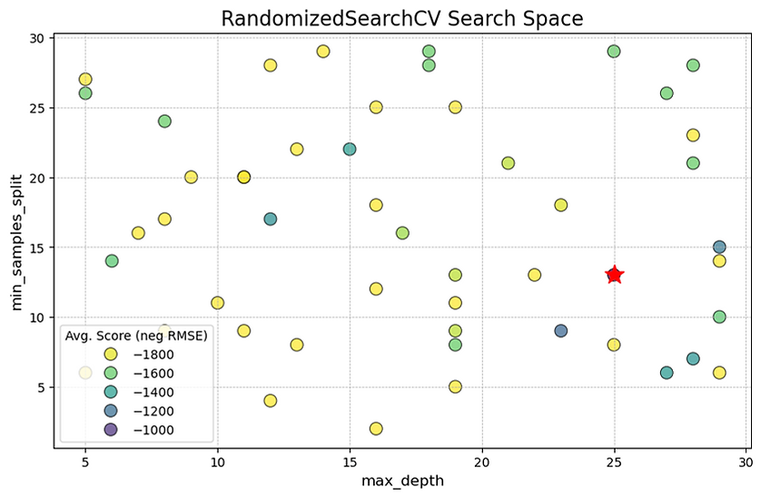
Unlike the rigid grid from the previous method, you can see how this search has tested random combinations of hyperparameters across a much wider range, shown by the scattered placement of the circles. The main finding is highlighted by the red star, which marks the best-performing model found by the search. This optimal combination included a max_depth of approximately 25 and a min_samples_split of about 13.

While the performance trend is less distinct than in the grid search due to the random sampling, we can still observe that many of the better-performing models (the darker blue and purple circles) tend to be located at higher max_depth values. This random approach allowed us to efficiently explore a broad search space without the computational cost of trying every single combination. It has successfully identified a high-performing region, suggesting that a relatively deep and complex tree is beneficial for this dataset, which aligns with our previous findings.

Halving Random Search

Now let's try the HalvingRandomSearchCV. Remember this is a high-speed, "tournament-style" hyperparameter tuning method. It finds the best parameter set by iteratively eliminating the worst performers. It starts by training a large number of random parameter combinations but it uses only a small fraction of the training data for each. After this initial round, it evaluates all the combinations and discards the worst-performing half. It then takes the surviving top half, doubles the amount of data they can train on, and repeats the process. This continues, with each round halving the number of candidates and increasing the resources for the survivors, until only the single best parameter combination remains, which has been fully trained on all available data.

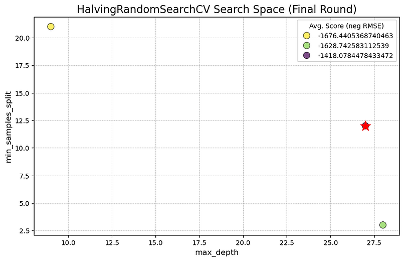
This plot shows the final round of our HalvingRandomSearchCV "tournament". The key takeaway, marked by the red star, is that the winning hyperparameter combination had a max_depth of approximately 27 and a min_samples_split of about 12. The three circles visible on the graph are the finalists that made it through all the previous elimination rounds. The dark purple colour of the winning point indicates it achieved the best performance score (the Negative RMSE value closest to zero), outperforming the other two survivors.

The reason there are so few points on this plot is that we are only looking at the conclusion of the search process. The HalvingRandomSearchCV method began with a much larger number of randomly chosen hyperparameter combinations. It trained all of them on a small subset of the data, evaluated their performance, and then discarded the bottom half. This process was repeated, with the surviving candidates getting progressively more data to train on in each round. The three points shown here are the "champions" that survived every elimination stage. This efficient, iterative process of culling the weakest options is why the method is so fast; it avoids wasting computational resources on unpromising candidates, which are filtered out long before this final round.

Now we've run all three search methods and seen how they sample their search space, let's see which one actually performed best on our data.

This comparison reveals a clear winner for our specific problem. RandomizedSearchCV delivered the best performance, achieving the lowest (best) RMSE score of 880.06. Despite trying more model combinations than GridSearchCV, it was also the fastest method at just 4.10 seconds. This demonstrates its key advantage: by randomly sampling from a wide range of values, it can efficiently explore the hyperparameter space and often find a superior combination in less time than a rigid grid search. For most tuning tasks, this blend of speed and effectiveness makes it the ideal starting point.

GridSearchCV acted as a reliable, if predictable, workhorse. It methodically tested all 36 specified combinations, guaranteeing that it found the best possible score within those narrow boundaries. Its final score of 880.97 was excellent and very close to the top result. However, its main drawback is its inefficiency. It spends just as much time on bad combinations as it does on good ones and cannot explore any "in-between" values, making it less suited for larger, more complex search spaces.

Counter-intuitively, HalvingRandomSearchCV performed the worst, delivering a much higher RMSE of 1418.08 and taking by far the longest time at 26.54 seconds. This provides a valuable lesson on choosing the right tool for the job. This method is designed for large datasets where training a single model is very time-consuming. It saves time by quickly eliminating bad models on small data subsets. The main issue is that HalvingRandomSearchCV is designed for problems where the number of samples is large, not necessarily the number of parameter combinations.

It works by training many models on a small subset of the data and progressively giving more data to the winners. In this tutorial, the training set is already very small (10% of the original data). The aggressive sub-sampling in the initial rounds means the models were trained on an extremely small number of data points, making their performance evaluations almost random. This not only leads to good models being eliminated but also makes the process inefficient as it struggles to find a stable performance signal. The method is most effective when we have a very large hyperparameter space to search and a dataset large enough that even a small fraction of it is sufficient to differentiate between good and bad parameter sets. On this small dataset, the initial evaluations were based on too few data points to be meaningful, making the elimination process almost random

Bayesian hyperparameter optimisation with Optuna

The final search method we'll explore is Optuna, a powerful open-source library designed specifically for hyperparameter optimisation. Unlike the "uninformed" approaches of GridSearchCV and RandomizedSearchCV, Optuna uses a sophisticated algorithm (a variant of Bayesian Optimisation called TPE) to learn from the results of past experiments. It builds a model of which hyperparameter combinations are likely to perform well and then uses this knowledge to decide which values to try next, focusing its search on the most promising areas of the hyperparameter space.

This (hopefully) allows us to find better solutions in fewer attempts. In theory it should be quicker than grid search as we don't need to test every combination of parameters. It should also find good combinations more efficiently than a random search. As each iteration of a random search is independent of the previous ones we could get unlucky and waste trials repeating very similar but less performant parameter combinations or under-exploring potentially promising areas of our hyperparameter space. Optuna tries to avoid this by carrying out a guided search based on the results of previous trials.

Optuna's API is a bit different from scikit-learn's. Instead of defining a static dictionary or "grid" upfront, we define the search space inside an objective function. The three core components we need to know are the 'study', the 'objective function', and the 'trial'. To understand how Optuna works, it helps to think of the whole process as a managed scientific experiment. Think of the study as the project director who oversees the entire operation. The objective function is the set of instructions for a single experiment and a trial is one specific run-through of those instructions.

We define the objective function for Optuna. It's a Python function that contains the complete recipe for a single trial: training and evaluating the model. Inside this function, we use the trial object to define our hyperparameter search space. For each hyperparameter, we ask the trial to suggest a value using methods like trial.suggest_int() for a range of whole numbers or trial.suggest_float() for a range of decimals. The trial object acts as a unique record for that single experiment, proposing a set of hyperparameter values based on the study's intelligent guidance. After the model is trained and evaluated using these suggested values, the objective function must return a final score, such as the RMSE.

The study object is the main controller that ties everything together. We create a study and tell it the overall goal—for example, to minimise the score returned by your objective function. When we tell the study to begin, it starts calling our objective function repeatedly. For each call, it passes a new trial object, collects the returned score, and updates its internal model. After learning from the outcome, it (in theory) makes an even more educated guess about which hyperparameters to suggest for the next trial, efficiently steering the search towards the optimal solution. Let's see how it works in practice.

This plot shows the results of our intelligent search using Optuna. The best-performing model, marked by the red star, was found with a max_depth of approximately 10 and a min_samples_split of about 2. As with the previous plots, each circle represents a single trial, and its colour indicates the performance, with the darker purplish colours representing a better score (a lower error).

What makes this plot particularly interesting is that you can see the evidence of Optuna's guided search strategy at work. Unlike a purely random search that would scatter points evenly, Optuna's approach has two phases visible here. First, it performs exploration, placing trials across the entire space—from the far left to the far right—to get a general sense of the performance landscape. Then, it begins exploitation. We can see a distinct cluster of trials on the left-hand side (around max_depth 5-7). This shows Optuna identifying this as a promising region early on and deciding to run more trials there to investigate further. This ability to learn from past results and focus on promising areas is what makes Optuna so efficient at finding optimal solutions.

Interestingly, the "intelligent" search from Optuna resulted in a significantly worse score of 1189.36 and was considerably slower than the random search. This highlights a crucial concept: an informed search can sometimes be misled. If Optuna gets unlucky with its first few trials and they land in a poor-performing area, its model may incorrectly rule out that entire region. It then focuses its remaining efforts on a different, suboptimal area, never finding the true best solution. One advantage of the RandomizedSearchCV is that it avoids this trap by continuing to sample broadly which in this case allowed it to find a better result.

Tuning all models

So far, we've focused on tuning a single DecisionTreeRegressor. Now, let's apply this process to our full suite of models from part 1. The code below creates a comprehensive run through of all the models. It begins by defining a list of all the different regression models, ranging from simple linear types to complex gradient boosting machines and neural networks. For each model, we define a "search space"— a range of potential hyperparameter settings to explore. We'll use the same pre-processing pipeline for each model so it's an even comparison between models.

Next we loop through every defined model. If a model has a hyperparameter search space, the we use RandomizedSearchCV to test 20 different random combinations and find the best one. For models that have their own built-in tuning mechanism (like LassoCV), we'll simply evaluate their default performance using cross-validation. Let's set a timer for each model tuning and then stores the results —including the model's name, its best performance score (RMSE) and the time taken at the end.

After running our comprehensive tuning pipeline, the results are clear: tree-based ensemble models, particularly those from the gradient boosting family, have decisively outperformed all other model types. The top four contenders—CatBoost, LightGBM, GradientBoosting, and HistGradientBoosting—all belong to this group. A significant performance gap separates them from the rest of the models, strongly suggesting that the relationships in our data are complex and non-linear, which is precisely where these models excel.

CatBoost ultimately clinched the top spot with the lowest Root Mean Squared Error (RMSE). However, this victory comes with a trade-off. If we also consider efficiency, both LightGBM and HistGradientBoosting present compelling alternatives. LightGBM achieved a score very close to the winner but in less than half the time. Meanwhile, HistGradientBoosting was the standout performer in terms of speed, securing a top-four score in just over seven seconds. This makes it by far the best choice when balancing accuracy with computational cost.

Further down the leaderboard, there's a noticeable drop-off in performance. The next best models were other tree-based ensembles like ExtraTrees and RandomForest. The linear models, while incredibly fast, simply couldn't capture the complex patterns in the data, leaving them far behind on accuracy. KNeighbors struggled the most, finishing in last place by a wide margin. In the end, our extensive tuning process has given us a decisive winner: for this problem, a gradient boosting model is undoubtedly the best tool for the job.

The eagle-eyed amongst you might have spotted that none of the highly tuned models actually managed to outperformed our baseline CatBoost model. This is likely in part to modern modelling packages having very good default parameters that are hard to improve upon but it might also be down to our pre-processing pipeline. Remember that we used the same pipeline for every model and it was a bit more tailored to the linear models as they struggle more with categorical data.

In the next section, we'll take our top performing models and not only tune each model's hyperparameters but also treat the pre-processing and target transformation steps themselves as things to be tuned. We will define a few competing pipeline options and have our search process discover the winning combination for each of our top-performing models. We'll also include different feature selection methods into the tuning pipeline too!

Tuning everything

The code below automates the process of finding the best possible machine learning model for our specific prediction task. We're essentially going to run 100 experiments where in each experiment, we try a different combination of data preparation techniques, modelling algorithms and hyperparameters to see which gives the best resuts. We'll use Optuna to keep track of all the trials and pipeline creations.

For every trial, it first decides how to prepare the raw data by choosing one of the predefined preprocessing methods. It then decides which predictive features (the data columns) are most important, testing different strategies for including or excluding them. After that, it selects one of three powerful modelling algorithms—CatBoost, LightGBM, or HistGradientBoosting—and tunes the hyperparameters to find the optimal configuration for that specific algorithm. Finally, it decides whether to apply a mathematical transformation to the target variable, which can sometimes improve model performance.

Once a complete pipeline is assembled for a trial, Optuna can evaluate its performance. Over time the hope is that it can hone in on the specific pre-processing steps, feature selection, model and hyperparameter space that give the best results. The advantage of tuning everything in one go is we can account for any interrelations between the different techniques e.g. a pre-processing pipeline that creates lots of dummy variables might pair better with a feature selection method, etc. From this process, we'll learn the single most effective strategy for solving our specific prediction problem, out of all the options we provided. It'll tell us what is the best way to clean and prepare our data was and whether it's better to use all our features or a select few. We'll also see which algorithm was best suited to our dataset's structure

Beyond just finding the single best model, this systematic approach also reveals deeper insights into the nature of our data. We might discover, for example, that one particular pre-processing method consistently outperforms others, regardless of the model used, suggesting it is particularly well-suited to our data's characteristics. We could also learn that aggressive feature selection is crucial for achieving high accuracy, or conversely, that it provides no real benefit. This allows us to move beyond guesswork and manual trial-and-error, providing a robust and efficient method for building a high-performing and well-understood predictive model. Let's kick it off and see how it does.

Our new, best model has a RMSE of 608 so represents a narrow improvement on our original, baseline model (609 RMSE)! You might be thinking that that was a lot of work for a tiny improvement and you'd be right. Depending on your use case often feature selection and hyperparameter tuning (especially when working with modern tree based package light LightGBM and CatBoost) can only result in small gains despite potentially training hundreds of models. On the other hand if your use case can benefit massively from small incremental improvements, then it can be worth pursuing.

Based on these results, the consistently best-performing models share a very clear and dominant recipe. The optimisation process quickly discovered a powerful combination of techniques, with subsequent trials largely refining the parameters of this successful formula rather than finding a completely new approach.

There is an exceptionally strong pattern regarding data preparation. Every single one of the top-performing trials used the imp_ordinal preprocessing pipeline. This method, which fills in missing values and converts categorical features into numerical order, was vastly superior. The alternative, imp_yeo_scale, which involves more complex transformations and scaling, consistently produced significantly worse results, often with an error rate almost double that of the best models.

Similarly, applying a log transform (LogTransform) to the target variable was absolutely essential for success (which is somethign we saw in part 1). All the best models, from the first top performer (Trial 1) to the final winner (Trial 92), utilised this transformation. This indicates that the target variable (diamond price) is likely skewed, and modelling its logarithm allows the algorithms to capture the underlying patterns far more effectively. Trials that did not use this transformation performed poorly.

The CatBoost model was the definitive winner. While LightGBM showed some early promise, CatBoost models consistently achieved and held the top spots throughout the latter 80 trials. It demonstrated a superior ability to find the best performance on this dataset. The optimal parameters for the winning CatBoost models generally involved a moderate tree depth (often between 5 and 7), a relatively high number of iterations (from 300 to over 900), and a learning rate typically in the range of 0.05 to 0.12.

The choice of feature selection was less critical than the other components, but a clear trend still emerged. The most successful models often used either no explicit feature selection (None) or a simple, model-based approach like SelectFromModel (which was used in the final best trial) and VarianceThreshold. Methods that aggressively remove features based on statistical scores, such as SelectKBest and SelectPercentile, proved to be high-risk; they were part of some reasonably good trials but also some of the worst, suggesting they sometimes remove valuable information. The best approach was to allow the robust CatBoost model to handle feature importance internally.

In summary, the optimisation repeatedly confirmed that the best approach is to use the imp_ordinal pipeline, apply a log transform to the price, and then train a CatBoost model with a moderate depth, letting the model itself determine feature importance without aggressive pre-filtering.

Nested Cross-Validation

Throughout our analysis, we've carefully kept a test set aside. All our crucial decisions—choosing the best model, the right preprocessing pipeline, and the optimal hyperparameters—were guided by performance scores from k-fold cross-validation on the training data. However, this process introduces a subtle but significant risk.

By running hundreds of trials and repeatedly selecting the configuration that scored best on our validation folds, we may have inadvertently begun to overfit the validation data itself. The winning score from our Optuna search might be overly optimistic because we chose that specific pipeline precisely because it performed well on those particular data splits. To get a truly unbiased estimate of how our entire tuning strategy will perform on new, unseen data, we can use nested cross-validation.

Nested cross-validation provides a more robust performance estimate by wrapping our entire hyperparameter search inside another, outer layer of cross-validation. The outer loop is responsible for providing an honest final score. It splits the data into several folds (e.g., 5), holding one fold out for evaluation and using the remaining folds for training. The inner loop is responsible for model tuning. For each training set created by the outer loop, we run our entire hyperparameter search (e.g., RandomizedSearchCV). This inner search performs its own cross-validation only on that subset of data to find the best model parameters.

The final nested score is the average of the scores from each outer loop evaluation. This estimate is less biased because the hyperparameter selection for each fold was performed without ever seeing the final evaluation data for that fold. Let's see how this works in practice. We will compare the score from a standard RandomizedSearchCV (which is potentially biased) with the more robust score from a full nested cross-validation.

In the code, the inner and outer loops are constructed using two separate KFold objects and are executed by nesting a RandomizedSearchCV object inside a cross_val_score function. The outer loop is created by the cross_val_score function, which uses the outer_cv object to split the entire X_train dataset into 5 folds. The primary role of this loop is to produce a final, unbiased performance score for the entire model tuning process. It doesn't tune hyperparameters itself; it only evaluates the outcome of the tuning that happens inside it.

The inner loop is defined by the RandomizedSearchCV object, specifically by its cv=inner_cv parameter. This loop's job is to perform the actual hyperparameter search. It operates only on the portion of data given to it by the outer loop in each iteration. Let's trace the data for the first iteration of the outer loop to see what's being measured.

Outer Loop Split: The outer_cv splits the full training data into 5 folds. It holds back Fold 1 (20% of the data) as the final validation set for this iteration and provides the remaining Folds 2, 3, 4, and 5 (80% of the data) as the training set.
Inner Loop Tuning: The RandomizedSearchCV (the search object) is now given only Folds 2-5. Inside this search:
- The inner_cv splits these four folds into their own 5 mini-folds.
- It then runs its 25 iterations of hyperparameter tuning. For each of the 25 hyperparameter combinations, it trains on 4 mini-folds and validates on 1 mini-fold, repeating this 5 times.
- After all iterations, it identifies the single best set of hyperparameters based on the average performance across the inner cross-validation.
Outer Loop Evaluation: The RandomizedSearchCV process finishes by training a final model using the best hyperparameters it just found on all of Folds 2, 3, 4, and 5. This single, optimised model is then evaluated once against the held-out Fold 1. The resulting RMSE score is the first of the five nested_scores.

This entire process is then repeated four more times, with each of the five outer folds getting a single turn as the held-out validation set. The final nested_score is the average of these five evaluation scores.

We can see from the results that there's a decent difference in the estimate of the model performance. As we'd expect, the outer folds score is worse than the inner fold. We only ran 25 random iterations so we the risk of overfitting to the validation set might not be too bad. However our earlier examples used a 100-trial guided search with Optuna that specifically took in information about the model performance on the validation set to pick its next set of parameters so was directly optimising and fitting on it

Let's take our best performing model from the nested CV and see how the different cross-validation scores compare to the test set. After the RandomizedSearchCV has finished, it stores the results of its search. The first two lines of the below code access these results:

search.best_params_: This retrieves a dictionary containing the specific combination of hyperparameters that achieved the best average score during the inner cross-validation loop.
search.best_estimator_: This retrieves the actual model pipeline, already fitted with the best hyperparameters on the full training data (X_train, y_train) during the .fit() call you made earlier.

While search.best_estimator_ is already trained, it's a common and good practice to explicitly refit it on the entire training dataset, as done with best_model.fit(X_train, y_train). This step ensures the final model has learned from 100% of the available training data before it makes its final predictions.

Finally, the code uses this fully trained final_model to predict outcomes on the X_test data. This is the first time the model has ever seen this data. The root_mean_squared_error function then compares these predictions to the true answers (y_test) to calculate the model's final score. This score is the most realistic estimate of how the model will perform on new, real-world data.

So it looks like our model actually performs much better on the test set than on either our inner or outer cross validation run! Whilst it's reassuring to see the model do better on the Test set ideally we want our cross-validation score to match our train-test scores as closely as possible so we know we've got a robust and generalisable pipeline.

What's likely happening in our case is that as the model only has 10% of the data to learn from it's struggling to learn and is underfitting. This is supported by the fact that each time the model gets a bit more data to train on, its performance improves. It has the least amount of data to train on in nested CV, a bit more in CV and then for the final model it has the full 10% to train on to predict the test. For larger data sets we wouldn't expect to have this issue but that comes with its own challenge that although nested validation is a great technique for getting as unbiased an idea of model performance as possible, it can be very time consuming to do.

Model Stacking: Creating a Super Learner

So far, our goal has been to find the single best-performing model through a process of feature selection and hyperparameter tuning. However, instead of choosing a single winning model, we could combine the strengths of several different ones into a 'super learner'. This is the core idea behind stacking, a powerful ensemble technique for creating a "super learner" that is often more accurate than any of its individual components.

Think of stacking as forming a committee of diverse experts. An economist, a sociologist and a data scientist will all approach a problem with different perspectives and make different types of mistakes. By combining their insights, a final decision-maker can arrive at a more robust conclusion. Stacking applies this logic to machine learning. We train a set of diverse "base models" and then train a final "meta-model" whose only job is to learn the best way to combine the base models' predictions.

The process involves two levels of models:

Train Base Models (Level 0): First, we train several different models on our data (e.g., a LightGBM, a RidgeCV, and an SVR).
Generate New Features: We use these base models to generate predictions on the training data. This is done carefully, using a cross-validation process to avoid data leakage. These predictions become a new set of features for the next level.
Train the Meta-Model (Level 1): Finally, we train a new, typically simple, model (like a linear regression) on the dataset created in the previous step. This meta-model learns the optimal weights to assign to each base model's "opinion." For example, it might learn that a gradient boosting model is usually the most reliable but that it should pay close attention when a support vector machine strongly disagrees.

The effectiveness of stacking hinges on the effectiveness of our underlying models but also their diversity. Combining five nearly identical models is fairly pointless as they will all make the same kinds of errors and the meta-model will have nothing new to learn. The goal is to choose base models that are as uncorrelated as possible in their predictions, meaning they approach the problem from different angles. A great strategy is to pick strong performers from different model "families" for example:

A gradient boosting model (e.g., LightGBM) that excels at complex interactions.
A linear model (e.g., RidgeCV) that captures the main linear trends.
A kernel-based model (e.g., SVR) or neural network that might capture other non-linear patterns.

Before building a stack, it's wise to check how correlated our potential base models are. A simple way to do this is to get the out-of-fold predictions for each model, combine them into a DataFrame, and calculate a correlation matrix. We ideally want strongly performing models with low correlation scores to each other. A heatmap is a great way to visualise this. If two models have a correlation of 0.98, they are making very similar predictions, and you should probably only include one of them. A model with a lower correlation (e.g. 0.85) is a much better candidate, as it brings a more unique "perspective" to the committee.

We know from our big tuning run earlier that our best models were CaBoost and the other boosting tree models. Let's try using the ExtraTrees and LassoCV to add a bit of diversity to our final stack. The code below generates out-of-fold predictions for each model and calculates the correlation matrix to assess their diversity for stacking.

Having said how important it is to have diverse models in our stack, our three candidate models are nearly perfectly correlated! This is likely due to our relatively small size of data and number of features. We could try adding some further models that performed worse e.g. support vector machine or neural network but for we'll carry on with these three for the demo.

The process begins by defining our base_estimators. This is our committee of experts, consisting of the three model pipelines we previously created. The StackingRegressor then orchestrates the entire operation. It manages the training of these base models and uses their predictions as input features to train the final_estimator, which we'll set as a RidgeCV model. The key steps are:

Level 0 (Base Models): The StackingRegressor first trains CatBoost, ExtraTrees, and LassoCV on the training data.
Level 1 (Meta-Model): It then trains the RidgeCV model, not on the original data but on the predictions generated by the Level 0 models.

You might wonder why we use a simple linear model like RidgeCV as the final decision-maker after using complex models like CatBoost. This is a deliberate and crucial choice for two main reasons. The base models have already done the heavy lifting of learning complex patterns from the original features. The meta-model has a much simpler job: to find the optimal weighted average of the base models' predictions. A simple linear model is perfectly suited for this task. Since the features for our meta-learner are already predictions from models themselves, its very easy to overfit our data if we pick too complicated a model. For example. If we used a complex model (like another CatBoost) as the meta-learner, it could memorise the specific errors and quirks of the base models on the training set but would not generalise well to new data. A simple, regularised model like RidgeCV is far less prone to this. It's forced to find a simple, robust combination of the base predictions without overfitting (hopefully) to their noise.

The other challenge with model stacking is to avoid data leakage. For example, our base models have already seen some of the training data to learn from and make predictions on. We want to take the out-of-fold predictions from our base models i.e. when they predicted on unseen data during training as the inputs to our meta-learner. To do this, we provide one layer of cross-validation via the cross_val_score function (the outer loop). The StackingRegressor itself automatically performs the inner cross-validation to generate the out-of-fold predictions for training the meta-model. We specify this inner CV strategy with the cv parameter inside StackingRegressor.

The Outer Loop (cross_val_score): This loop's only job is evaluation. It splits our training data 5 times. In each run, it trains the entire StackingRegressor on 4 folds and scores it on the 1 held-out fold. The final RMSE we see is the average of these 5 scores, giving you a robust estimate of how the whole stack will perform.
The Inner Loop (cv inside StackingRegressor): This loop's job is to generate clean training data for the meta-model. Within each run of the outer loop, the StackingRegressor performs its own internal cross-validation on the training data it received. It trains the base models on a portion of this data and gets their predictions on the rest, ensuring that a model's prediction for a data point is never generated by a version of itself that was trained on that same data point. This process generates "out-of-fold" predictions, which are then used as an unbiased training set for the RidgeCV meta-model.

Let's see how it all works in practice.

Great, so it looks like our stacked ensemble achieved a final RMSE of ~600 which is a decent improvement over our previous best-tuned individual model. This is a resounding success and a powerful demonstration of why stacking is a go-to technique for winning machine learning competitions and building state-of-the-art models.

Interpretable models with SHAPLEY values

With our stacked model, we've successfully built a powerful model that can predict diamond prices with a high degree of accuracy. However, we're now faced with the classic "black box" problem. We know what our model predicts, but we don't know why. Why did it give one diamond a high price and another a low one? Which features are the most influential, and precisely how do they affect the final prediction? At least with our CatBoost model we could ask it for what feature it found important. Answering these questions is critical for trusting our model, debugging it, and explaining its decisions to others. For this, we'll turn to SHAP (SHapley Additive exPlanations), a state-of-the-art method for explaining the output of any machine learning model.

SHAP is based on a concept from cooperative game theory called Shapley values. The core idea is to treat a model's prediction as a "game" where the features are the "players" and the final prediction is the "payout." SHAP calculates the fairest way to distribute this payout among the features, giving us the exact contribution of each feature to each individual prediction.

For any single prediction, SHAP values tell us how much each feature has pushed the model's output away from the average prediction. Starting with a base value, which is the average prediction calculated over our entire training dataset, a positive SHAP value for a feature means it pushed the prediction for that specific diamond higher than the average. Conversely, a negative SHAP value means that feature pushed the prediction lower. The key property of SHAP is that these contributions are perfectly additive. For any single prediction, the formula is simply:

Final Prediction = Base Value+∑(SHAP values of all features)

This makes SHAP an incredibly powerful tool for understanding exactly how our model arrived at its decision for any given input.The following code will first fit our stacking_regressor on all the training data. Then, it will calculate the SHAP values, which can take a few minutes as it's a computationally intensive process. Finally, it will generate a series of plots, each designed to give us a different insight into our model's behaviour.

Since our stacked model is very much a black box, we'll use the KernelExplainer which is a model-agnostic tool, which means it doesn't need to know the internal workings of our stacking regressor. Instead, it probes the model from the outside. For each single prediction we want to explain from our test set, it plays a clever "what-if" game. It creates numerous new data points by forming different "coalitions" or subsets of the original features. When a feature is "absent" from a coalition, the explainer substitutes its value with one drawn from the background data. We then pass all these new perturbed data points to our model using the predict_fn_stack function and record the outputs. By analysing how the prediction changes as features are included or excluded, the explainer fits a simple, interpretable linear model that is only valid for that specific prediction. The weights of this local model are the SHAP values, which represent each feature's contribution.

We can see that it took 6 minutes just to process 200 test set observations! We use samples simply because the KernelExplainer process is very slow. Running it on our entire dataset would likely take far too long to be practical. The 100 training values (X_train_summary) serve as our background dataset. Its purpose is to provide a baseline for what feature values typically look like. The KernelExplainer works by replacing features with values from this background set to simulate their "absence." A good background set should be a representative sample of the training data (e.g., the k-means centroids) to provide a realistic baseline for these substitutions. When the explainer simulates a feature's "absence" during its what-if analysis, it needs a realistic value to plug in its place. By sampling from these 100 representative instances, we give the explainer a context to accurately measure the impact of the features that are present.

The 200 test values (X_test_sample) are the specific instances we want to explain. We're not explaining the entire model at once, but rather calculating SHAP values for each of these 200 individual predictions. The final output, shap_values, will contain a detailed explanation showing the feature contributions for every single one of these 200 predictions, helping us understand why our model made the decisions it did. First, we'll look at the model's behaviour from a global perspective. The bar plot gives us a straightforward ranking of feature importance. It answers the question: "Overall, which features have the biggest impact on the model's predictions?"

The beeswarm plot provides a much richer view. Not only does it rank the features by importance, but it also shows the direction and magnitude of each feature's effect for every point in our sample. For example, we can see how high values of a feature (shown in red) and low values (shown in blue) impact the prediction. This helps us understand not just that a feature is important, but how it's important.

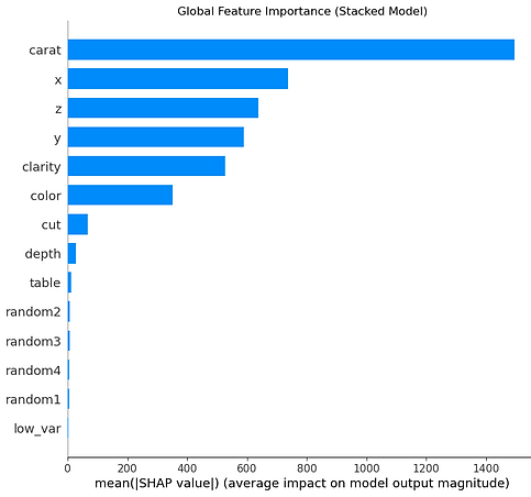
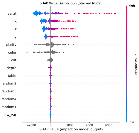
These plots offer a comprehensive view of how our stacked model makes its predictions. The chart on the left tells us which features are most important overall, while the one on the right explains how each feature's value affects the final prediction.

The bar chart on the left ranks our features based on their average impact on the model's output. A longer bar signifies a more influential feature. It's immediately clear that carat is the most dominant feature by a wide margin, having more than double the impact of the next feature. Following this are the diamond's physical dimensions, x, z, and y. Features like clarity and colour have a moderate and noticeable impact. It's also reassuring to see that features like cut and depth, along with the random and low_var noise features we added, have very little importance. This is a great sign that our model is robust and has correctly learned to ignore irrelevant information.

The "beeswarm" plot on the right gives us a much richer understanding. Each dot represents a single prediction from our data. Its position on the horizontal axis shows how much that feature pushed the prediction higher (a positive SHAP value) or lower (a negative SHAP value). The colour of the dot indicates whether the feature's original value was high (red) or low (blue).

For carat, the relationship is crystal clear: high carat values (red dots) consistently have large positive SHAP values, meaning they strongly increase the predicted price. Conversely, low carat values (blue dots) push the prediction down. The dimensions x, z, and y follow the same intuitive pattern. For clarity and colour, we can see that higher values on the feature scale (likely representing better clarity or colour grades) tend to increase the price, whereas lower values decrease it. Finally, just as we saw in the first chart, the random and low_var features are clustered tightly around the zero line, confirming they have no real impact on the model's output, which is precisely what we'd hope to see.

Next, we'll zoom in to the local level and explain a single, individual prediction. The force plot is a brilliant way to visualise this. It starts with the "base value," which is the average prediction across our entire dataset. Then, it shows how each feature of that specific diamond acts as a "force," pushing the prediction higher (in red) or lower (in blue) until it reaches its final value. This allows us to tell a complete story for any prediction our model makes.

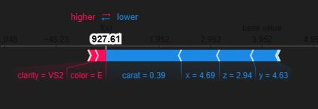
This SHAP force plot explains why our model made a single prediction of £927.61. It shows a "tug-of-war" between features that pushed the price higher (in red) and features that pushed it lower (in blue). The model starts with a base value (around £3,952 on the grey axis), which is the average prediction for all diamonds.The bold number, £927.61, is the final price predicted for this specific diamond. Features in red are pushing the prediction up from the base value. The larger the red block, the stronger its positive impact. Features in blue are pushing the prediction down. The larger the blue block, the stronger its negative impact. The model predicted a price of £927.61, which is much lower than the average.

The main reason for this low price is the diamond's small size. The carat = 0.39 feature provides the largest push downwards, significantly lowering the price. The small physical dimensions (x, z, and y) also contribute to the lower price.On the other hand, the diamond has good quality characteristics. Its clarity = VS2 and color = E are both positive attributes that push the price higher. However, the combined positive effect of these two features is far outweighed by the massive negative impact of the diamond's small size.

Let's generate an interactive force plot for our entire sample, which stacks all the individual explanations on top of each other. This is a powerful way to see patterns in how the model makes decisions across many different predictions.

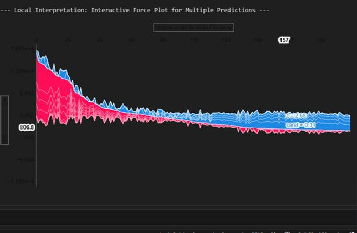
This chart is a "force plot" for multiple predictions, which stacks the individual explanations for all the predictions in our sample on top of each other. It's a handy way to get a bird's-eye view of our model's behaviour across a whole group of data points. The plot arranges each individual prediction from our X_test_sample along the horizontal axis. By default, SHAP clusters predictions with similar explanations together but this one is ordered by predicted value. This allows us to quickly see which features consistently drive high prices and which ones drive low prices, giving you a powerful overview of the model's logic at its extremes.

The vertical axis represents the model's output value, with the centre line being the average prediction, or base value. The wavy line that separates the red and blue areas is the model's final prediction for each specific instance. The real insight comes from the coloured areas. The red zones show the combined impact of all the features that are pushing the prediction higher than the average. The blue zones show the combined impact of features pushing the prediction lower. In our chart, it's clear there's a cluster of high-value predictions on the left, driven by positive factors, and a larger group of lower-value predictions on the right, driven by negative factors.

What makes this chart so powerful is its interactivity. We can hover our mouse over any vertical slice to see a pop-up of the specific force plot for that single prediction, breaking down exactly how it was made. In the screenshot, we're looking at instance #157. We can also move our mouse over one of the coloured bands, like the one for carat=0.31, and the chart will highlight that feature's impact across all the predictions. This lets us see at a glance how a single feature influences the entire sample, making it an incredible tool for exploring our model's logic.

Finally, the dependence plot helps us dive deeper into the effect of a single feature. We'll look at carat to see how its SHAP value (its impact on the prediction) changes as the value of carat itself changes. This can reveal complex, non-linear relationships.

The vertical spread of points in this plot also hints at interaction effects. SHAP automatically colours the dots by the feature it believes has the strongest interaction with carat, helping us discover which features work together to influence the final prediction.

This SHAP dependence plot shows us how the carat feature's value affects the model's predicted price for a diamond. It reveals not only the direct impact of carat weight but also its interaction with the diamond's length, represented by the feature x. The plot clearly shows a strong, positive relationship between a diamond's carat weight and its impact on the price. Each dot on the chart is a single diamond from our sample. The horizontal position shows its actual carat weight, and the vertical position shows its SHAP value—how much that carat weight pushed the prediction higher or lower. We can see that diamonds with a low carat weight (below about 0.9) have negative SHAP values, meaning they actively reduce the predicted price from the average. As the carat weight increases, its SHAP value also increases, meaning heavier diamonds have a strong positive impact on the predicted price.

The colour of each dot reveals an interaction effect with another feature, which SHAP has automatically chosen as x (the diamond's length). The colour bar shows that blue dots represent diamonds with a small x value, while the pink and red dots represent diamonds with a larger x value. The plot confirms what we'd intuitively expect: low carat diamonds are physically small (blue dots on the left), and high carat diamonds are physically large (red dots on the right). This strong correlation between carat and x means that both features work together to drive the price up.

As our stacked model didn't have an inbuilt form If we'd used the CatBoost model on its own, we could have used SHAP's optimised TreeExplainer, which unlocks significant extra functionality and is much more efficient. The KernelExplainer we used for our stacked model is a fantastic model-agnostic tool, but it's slow. It works by repeatedly making small changes to the input data and calling the model's predict function to see how the output changes. In contrast, the TreeExplainer is specifically designed for tree-based models like CatBoost. It understands the model's internal structure and can calculate the exact SHAP values in a fraction of the time without needing to call the predict function repeatedly. This means we could have calculated SHAP values for our entire test set in seconds, rather than waiting minutes for a small sample.

The most powerful feature we missed out on is the ability to calculate SHAP interaction values. This is an advanced capability, exclusive to tree-based models, that goes a step further than standard SHAP values. While a standard SHAP value tells you a feature's total contribution, the interaction value breaks this down. It shows you the feature's main effect and how much of its contribution came from "teamwork" or interaction with every other feature. This allows us to answer much deeper questions, such as "How much of carat's importance is due to its interaction with clarity?" With interaction values, we could have created more advanced dependence plots and a summary plot of the top interaction effects, giving us a far more detailed understanding of how our features work together in the model.

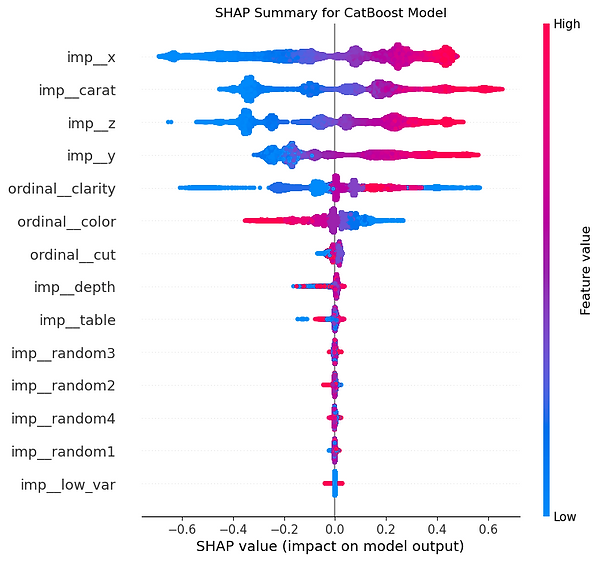
This chart is a SHAP summary plot for our CatBoost model, and it's telling us which features the model considers most important and exactly how they influence its price predictions. It effectively combines feature importance with the real-world effects of those features.

Each dot on the plot represents a single prediction for a diamond in our dataset. The features are ranked by importance from top to bottom. The horizontal position of a dot shows whether that feature's value pushed the predicted price higher (to the right) or lower (to the left). The colour of the dot tells us if the feature's value for that diamond was high (red) or low (blue). From this, it's immediately clear that the most influential features are the diamond's physical dimensions and weight: imp__x (length), imp__carat, imp__z (depth), and imp__y (width).

For these top features, the relationship is very straightforward and logical. We can see that high feature values, shown as red dots, consistently have positive SHAP values, meaning larger and heavier diamonds lead to a higher predicted price. Conversely, low feature values, shown as blue dots, have negative SHAP values, significantly lowering the predicted price. The next most important features are the ordinally encoded clarity, color, and cut. For clarity, we can see a trend where higher encoded values (better clarity) tend to increase the price. The effect of color is a bit more mixed, but it still has a clear impact.

Finally, a very reassuring sign is at the bottom of the plot. All the random features and the low_var feature are clustered tightly around the zero line. This tells us that our CatBoost model has correctly learned that these features are useless and has given them virtually no importance in its decision-making process.

As well as tree-based interpreters, SHAP also has a LinearExplainer which we can use with our best performing linear model, the LassoCV.

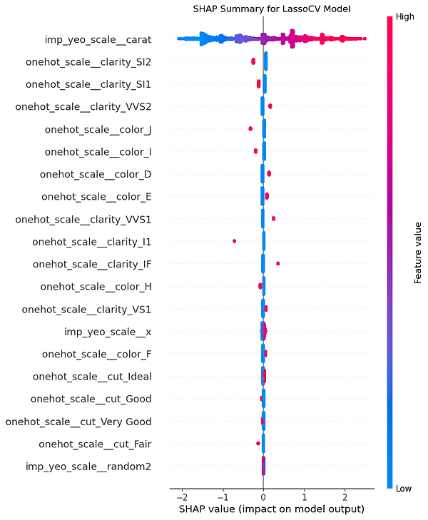
This SHAP summary plot explains how our LassoCV model makes its predictions. It's quite different from the CatBoost plot because it perfectly illustrates the unique behaviour of a Lasso regression model.

The plot shows us which features the model uses and how they affect the predicted price. We can see that imp_yeo_scale__carat is overwhelmingly the most important feature. The trend is very clear: high carat values (the red dots) have a large positive SHAP value, meaning they strongly increase the price, while low carat values (the blue dots) have a large negative SHAP value, strongly decreasing the price. This is the primary driver of the model's predictions.

What's most revealing about this chart is the effect of the Lasso regularisation. Lasso is designed to simplify a model by shrinking the importance of less useful features, often all the way to zero. We can see that effect in action here. Most of the one-hot encoded features, such as those for the different cut qualities, have all their SHAP values sitting exactly on the zero line. This means our Lasso model has decided they're not predictive enough and has completely ignored them.

Only a sparse handful of other features have survived this selection process. For example, the presence of a poor clarity grade like clarity_SI2 (where its value is 1, shown as a red dot) has a negative impact on the price, which makes sense. Conversely, top grades like clarity_IF have a small positive impact. In essence, this plot shows us that the Lasso model has built a very simple, sparse model that relies almost entirely on carat and just a few specific categorical flags to make its predictions.

Summary

In this tutorial, we've moved on from building a robust baseline model to exploring a range of advanced techniques to enhance its performance and interpretability even more. We've looked at various feature selection methods and how to correctly implement them within a cross-validation framework to prevent data leakage. We've looked at hyperparameter tuning, comparing different search strategies and discovering that while tuning can provide a boost, modern algorithms like CatBoost often have powerful default settings that are hard to beat. Our most significant performance gain came from model stacking, where we combined several diverse models into a "super learner" that outperformed any single model on its own.

Finally, we addressed the "black box" problem by using SHAP to interpret our final model's predictions. This allowed us to understand exactly which features were driving the model's decisions and by how much, providing transparency and building trust in our results. The key takeaway is that while significant gains often come from better data and feature engineering, a systematic approach involving robust validation, feature selection, hyperparameter tuning and ensembling can squeeze out extra performance. The ability to also interpret and explain a model's predictions can also sometimes be just as important as its predictive accuracy.

Intro

Stacking

Feature Selection

SHAP

Hyperparameters